3. VISIBLE IMAGER CALIBRATION

3.1 Overview

This section describes the calibration procedure that is applied to THEMIS-VIS raw Experiment Data Records (EDRs) in order to generate Reduced Data Records (RDRs). This section is provided by T. H. McConnochie and J. F. Bell, Cornell University (Calibration and In-Flight Performance of the Mars Odyssey THEMIS-VIS Instrument, Journal of Geophysical Research – Planets, submitted December 2005).

We describe the calibration and performance of the Mars Odyssey spacecraft’s Thermal Emission Imaging System Visible-Imaging Subsystem (THEMIS-VIS), and present comparisons with other instruments in order to validate the results. The main challenge to the THEMIS-VIS calibration process is the significant amount of stray light that accumulates during both integration and readout. The stray light is influenced by scene elements outside of the field of view of the THEMIS-VIS detector, and so its magnitude can only be estimated. As a result, residual stray light artifacts are common in calibrated THEMIS-VIS images, and are especially prominent when the exposure time is short, or the scene contrast is high. Nevertheless, our absolute 2s calibration uncertainty for the central region of the most frequently used THEMIS-VIS channel – the 654 nm band – is better than 5% for all but the shortest exposures times, and our comparisons with Hubble Space Telescope and Mars Exploration Rover measurements show no evidence of systematic calibration inaccuracies.

3.2 Introduction

The Mars Odyssey spacecraft’s Thermal Emission Imaging System (THEMIS) consists of two independent multispectral imagers sharing a single telescope – a nine-band mid-infrared microbolometer arrary (THEMIS-IR), and a five-band visible/near-infrared interline-transfer CCD (THEMIS-VIS). THEMIS has been acquiring visible and infrared images from Odyssey's 400 km circular polar orbit since February 2002, and has already provided important new insights about the geology and evolution of the martian surface (e.g., Christensen et al., 2003; Titus et al., 2003; Pelkey et al., 2003, 2004; Milam et al., 2003). Details of the THEMIS design, including THEMIS-IR, and the optics shared by both subsystems, can be found in Christensen et al. (2004). The purpose of this paper is to describe and evaluate the calibration of THEMIS-VIS, and to describe aspects of the instrument design and on-orbit performance which are directly related to the calibration.

THEMIS-VIS is one of several visible light instruments currently in operation in Mars orbit. Of these, the Mars Orbiter Camera (MOC) on the Mars Global Surveyor (MGS) orbiter (Malin et al., 1992), and the High-Resolution Stereo Camera (HRSC) on the Mars Express orbiter (Neukum and Jaumann, 2004) are most similar to THEMIS-VIS. The OMEGA imaging spectrometer on Mars Express (Bonello et al., 2004), the visible-band bolometer detectors of the Thermal Emission Spectrometer (TES) on MGS (Christensen et al., 1992), and the Wide-Field Planetary Camera 2 (WFPC2), Advanced Camera for Surveys (ACS), and Space Telescope Imaging Spectrometer (STIS) (e.g., Bell, 2003) on the Hubble Space Telescope (HST) are also currently providing (or have recently provided) visible-light coverage of Mars, but at significantly lower resolutions than MOC and HRSC.

MOC acquires monochrome images at scales as small as ~1.5 m and two-color imagery at regional and global scales from a circular, 400 km altitude, 2:00 p.m. local solar time Sun-synchronous orbit (Malin et al., 1992). HRSC provides stereo imagery and 4-channel color from a highly elliptical orbit with a best resolution of ~50 meters per pixel (Neukum and Jaumann, 2004). Both MOC and HRSC are line-scan cameras, which use linear Charge-Coupled Device (CCD) arrays to obtain information along one axis, and spacecraft ground track motion perpendicular to the CCD array direction to obtain the other spatial axis. THEMIS-VIS acquires monochrome or color images in any combination of its five bands with resolution modes of 18, 36, and 72 meters per pixel from its circular, 400 km, approximately Sun-synchronous orbit at typical local solar times of 4:00 p.m. to 5:00 p.m. The filter bandpasses have a FWHM of roughly 50 nm and are centered at 423, 540, 654, 749, and 860 nm. Fig. 1a shows the THEMIS-VIS bandpass profiles. Unlike MOC and HRSC, THEMIS-VIS is a 2-D array framing camera – all 1024 x 1032 CCD pixels are exposed simultaneously. However, spacecraft ground track motion is also used to expand the spatial coverage of acquired imaging sequences. While THEMIS-VIS is not designed to provide stereo capability, a limited amount of information on the altitude and cross-track velocity of high clouds can be derived by co-registering overlapping frames acquired at slightly changing viewing geometries over the course of a color imaging sequence (McConnochie et al., 2004).

THEMIS-VIS was found to have a serious problem from stray light contaminating the detector signal both during integration and during the CCD readout. Stray light accumulation during integration affects the entire array, but is most noticeable as broad and brighter stripes of additional signal near the edges of uncalibrated images. Stray light accumulation during the readout process creates an additive offset, and an effect similar to the "electronic shutter smear" seen in some shutterless CCD imaging systems, both of which are proportional to scene brightness but independent of the exposure time. Most of this paper is focused on the removal of both forms of stray light contamination from THEMIS-VIS images.

This paper describes and evaluates the process by which the radiance-calibrated data stored in the NASA Planetary Data System (PDS) THEMIS-VIS Reduced Data Records (RDRs; accessible via the internet at http://themis-data.asu.edu/) is generated from the raw PDS Engineering Data Records (EDRs). (Note that THEMIS-VIS RDRs are not geometrically calibrated. This paper does not address geometric calibration.) We begin by describing the relevant operational details of THEMIS-VIS, as well as our preferred model for the stray-light contamination mechanisms. We then discuss each step of the EDR-to-RDR calibration process. Finally, we evaluate the calibration by comparing the derived THEMIS-VIS radiances to HST results, as well as to the surface-based multispectral measurements provided by the Mars Exploration Rovers’ Panoramic Cameras (Pancams).

3.3 Operational Details and Labeling Conventions

VIS uses a Kodak interline-transfer CCD. For each column of photosites, there is a masked vertical register (v-register) adjacent to it. At the start of a THEMIS-VIS exposure, any charge accumulated on the detector is flushed. Charge accumulated in the photosites is transferred to the adjacent v-registers twice during the commanded exposure period – once at the midpoint and once at the end. The v-registers are masked to minimize accumulation of photo-electrons during readout. During the readout process, beginning immediately after the second photosite charge transfer, the charge is shifted "downstream," i.e., down the v-registers and transferred to the CCD’s horizontal register (h-register) one row at a time. The h-register will be considered to be at the "bottom" of the detector array in this paper, so that "down" and "downstream" are in the same direction. That is, if one row of pixels is said to be below or downstream of another row of pixels, then the row that is “below” or “downstream” is closer to the h-register. With this convention, the direction of spacecraft motion (south on the afternoon side of the orbit) is always “down.” We number rows starting from zero at the bottom. Note, however, that the opposite row ordering convention is used in PDS EDR and RDR products.

Physically, the THEMIS-VIS CCD detector has 1032 columns and 1024 rows. The 5 THEMIS-VIS filters are strips that are 1032 columns wide and approximately 200 rows tall and are bonded directly to the detector. The front of the CCD housing is covered by a window, which therefore falls between the filter strips and the telescope optics, and which influences the overall spectral response in each THEMIS-VIS band. Figure 1a gives the spectral response through each THEMIS-VIS filter with the spectral throughput of the CCD window included. The spectral response of each filter by itself turns out to be important, as we will show, for predicting the magnitude of stray light contamination, and is therefore plotted in Figure 1b.

In this document, as in the EDR and RDR labels on the PDS files, the filters are labeled "filter 1", "filter 2", …"filter 5" in order of their position on the detector array, with filter 1 at the bottom, closest to the h-register. In this naming scheme, "filter 1" is 860 nm, "filter 2" is 425 nm, "filter 3" is 654 nm, "filter 4" is 749 nm and "filter 5" is 540 nm. An alternate filter designation exists, using the labels "band 1", "band 2", …"band 5" to refer to the filters in order of increasing center wavelength [425, 540, 654, 749, 860 nm]. Figure 2 shows the THEMIS-VIS focal plane with “filters” f and “bands” k labeled.

The groundtrack of the Odyssey spacecraft runs approximately parallel to the detector columns. This allows multispectral images to be acquired using a timed sequence of THEMIS-VIS exposures. Any combination of one or more filters can be acquired by selectively reading out only those rows that correspond to the desired filters. Thus, a single THEMIS-VIS exposure can contain any or all of the five filters. We refer to the portion of an exposure that contains data for a single filter as a "framelet." All exposures in a sequence have the same exposure duration, and all filters in an exposure must have the same exposure duration, and so all framelets in a given THEMIS-VIS sequence have identical exposure durations.

The different filter framelets in a full-frame THEMIS-VIS exposure cover different regions of the Martian surface (nominally about 3.6 km apart for adjacent filters), hence the need for a sequence of multiple exposures to build up a multispectral image using spacecraft downtrack motion to image the same parts of the surface through different filters (and thus at slightly different times). The exposure sequences are designed so that all filters end up with the same number of framelets, and so that when a filter moves past the targeted region of the surface, it is no longer read out, meaning that the first and last several exposures of an imaging sequence will have a smaller number of filters read out than exposures in the middle of a sequence. Figure 3 illustrates the way that the framelets of a series of exposures map onto the Martian surface and can be arranged to form a continuous image strip for each filter.

The delay between exposures within a THEMIS-VIS imaging sequence is set so as to maximize the areal coverage of an imaging sequence while allowing for adequate overlap between adjacent framelets of the same band. A 1 second delay leads to a typical overlap of between 10 and 20 detector pixels (depending on the surface elevation and the angle of the planet’s rotation relative to the groundtrack) when projected onto the martian surface. One side effect of this overlap is that framelets of different bands are not exactly spatially coincident when map projected, meaning that framelet boundaries (and calibration artifacts associated with those boundaries) for different bands are in different positions in mapped data, and that the total area covered by lower-numbered filters within a sequence is offset relative to that covered by higher-numbered filters by a number of pixels equal to the framelet-to-framelet overlap multiplied by the difference in filter number. The delay between exposures is given by the “INTERFRAME_DELAY” keyword in the THEMIS-VIS PDS headers. A standard interframe delay of 1.00 seconds was for used image numbers up through V14885012. The standard interframe delay was changed to 0.90 seconds beginning with V14886001.

Rows and columns near the edges of the filters are always cropped during readout. The result is that each framelet has dimensions of 1024 by 192 detector pixels. The rows that are cropped are referred to henceforth as inter-framelet rows. When THEMIS-VIS EDR “cubes” are generated (3-dimensional data sets containing both spatial and spectral information, in PDS “QUB” file format), the THEMIS-VIS exposures in a sequence are broken up into their constituent framelets and re-assembled so that each framelet’s position in the cube corresponds roughly to its spatial location on the surface of the planet. Thus, for a given filter, the corresponding plane of the EDR QUB is generated by concatenating the framelets from top to bottom in the order in which they were acquired. Assuming no spatial summing (spatial summing is discussed below), and using the PDS row ordering convention (opposite that used elsewhere in this paper), the first (top) framelet goes in EDR rows 0 – 191, the second in EDR rows 192 – 383, etc.. Within a given EDR QUB plane, we assign the framelets a number, m, starting from the top, with the first framelet acquired in a given filter being m = 0.

The procedure for removing stray light accumulated during readout requires that all of the framelets from a given exposure be grouped together. Consider a framelet at position m₀ taken through filter number f₀. The position m₁ of the framelet taken through filter number f₁ that was acquired in the same exposure as framelet (m₀, f₀) can be found by the following equation:

. (1)

If m₁ < 0 or m₁ ³ n, where n is the number of framelets in each filter in the EDR cube, then there was no framelet of filter f₁ acquired in the same exposure as framelet (m₀, f₀). Note that equation (1) is written in terms of filter numbers, which are, as mentioned previously, not the same as band numbers. Note also, however, that the EDR and RDR QUB planes are stored in band order, not in filter order, and the location of each filter within the EDR and RDR cubes is given by the BAND_BIN_FILTER keyword in the PDS labels. Figure 4 shows all five planes of the EDR from a five-band THEMIS-VIS imaging sequence with each framelet labeled according to its band number k, filter number f, framelet number m, and exposure number a. Exposure number a is defined so that it is equal to m for the lowest numbered filter in a given EDR or RDR; thus:

. (2)

THEMIS-VIS can operate in any of three spatial summing modes. The preceding discussion has assumed summing mode 1, i.e., no spatial summing, for clarity. In summing modes (i.e., for spatial summing factors of) 2 and 4, the THEMIS-VIS pixels are binned 2 x 2 and 4 x 4, respectively. This creates framelets with 512 columns by 96 rows, or 256 columns by 48 rows, respectively. Summing mode 1 has a typical pixel scale of 18 meters on the martian surface for a nadir-pointed viewing geometry. Thus, summing modes 2 and 4 have nadir-pointed pixel scales of 36 and 72 meters per pixel. To date, the martian surface has been targeted solely in the nadir-pointed configuration, so actual pixel scales will vary only slightly from the values quoted here.

The amount of time required to read out a single THEMIS-VIS exposure depends both on the spatial summing mode and on the number of filters being read out. Each framelet of an exposure requires 141, 76, or 39 msec to read out, for summing modes 1, 2, and 4, respectively. A small amount of time (~ 4 msec) is also required to "dump" the charge from each filter that is not being read out. About 0.2 msec is required to dump each group of the inter-framelet rows, which are never read out. So, for example, it takes 703 msec to complete the readout process when summing mode 1 data from all five filters is being acquired. Since this readout time is long compared to the ~5-10 msec typical exposure time, the opacity of the masks that protect the v-registers from photo-electrons, as well as the amount of time that each row of data spends in the v-registers during readout, are crucial factors for the THEMIS-VIS calibration process. And since THEMIS-VIS quickly dumps the charge in filters not being read out, the amount of time a given row spends in the v-registers depends not only on its distance from the h-register, but also on which of the filters that are below it on the array are being read out.

Correcting for stray light and dark current accumulation during readout requires knowledge of the timing for each data pixel as it is clocked down the v-registers to the h-register during readout. For pixels in a given filter, this timing depends on which of the lower-numbered (closer to h-register) filters are being read out in a particular exposure, and which are being dumped and not read out. Pixels in filter number f have 2^(f-1) possible timing "paths" during readout (e.g., for filter 3, these are the read out filter combinations [3,2,1], [3,2], [3,1], and [3]). The total number of possible paths is therefore

. (3)

These 31 possible paths will henceforth be referred to as "filter paths." Each path is given a filter path code, F. For a given filter with filter number f₀, F is determined by:

. (4)

A filter is included in an exposure if both of the following are true: (1) the filter is present in the EDR; and (2) the framelet position m of the filter (as calculated from equation (1)) satisfies m₁ < n and m₁ ³ 0, where n is the number of framelets of each filter in the EDR cube.

The calibration process is also influenced by the manner in which the THEMIS-VIS electronics perform spatial summing and store the data. The number of pixels summed in the “horizontal” direction (along rows) is always equal to the number of pixels summed in the “vertical” direction (along columns), but the spatial summing in each direction is performed in a different manner. Vertical summing, if any, is performed in the h-register. The charge from the appropriate number of v-register pixels is simply added together into each h-register site, and the h-register sites are then passed to the analog-to-digital (A-to-D) converter and represented as digital (“data number” or “DN”) values with a gain measured at 25.4 electrons per DN. An additive bias equal to 104 DNs is removed at this stage, after which DN values can range from 0 to 2047 (i.e., 11 available bits) regardless of the spatial summing mode. At this point, summing has only been performed along the vertical axis, and the DN values represent charge from a number of pixels equal to the spatial summing factor. That is, for a given exposure time and scene brightness, 2x2 summing gives, neglecting charge accumulation during readout, twice as much h-register charge, and thus a DN value which is larger by a factor of two.

Next, horizontal summing is performed on these DN values by THEMIS-VIS onboard software, but now the appropriate number of pixels are averaged rather than summed, so that DN values in the 0 – 2047 range remain in the 0 – 2047 range. Thus, considering the total effect of the two disparate steps of the spatial summing process, the values returned by THEMIS-VIS with spatial summing are, with a given scene brightness and exposure time, still only larger by a factor equal to the spatial summing factor (rather than to the spatial summing factor squared) once readout-accumulated charge has been removed, and the amount of exposure time required to reach saturation of the available 0 – 2047 DN representation range is correspondingly less by a factor equal to the spatial summing factor.

Before the THEMIS-VIS data are sent to the Odyssey spacecraft flight computer for storage and eventual downlink, the 0 – 2047 11-bit DN values are compressed into a 0 – 255 8-bit range using a square-root encoding algorithm. It is important to note that 0 – 255 square-root encoded data is preserved in the EDR, that the encoding is non-linear, and that therefore the encoding must be reversed before the THEMIS-VIS EDR data is used in any quantitative way. (See Table 5.)

The number of framelets in any THEMIS-VIS imaging sequence is limited by the 3.8 megabyte capacity of the THEMIS-VIS instrument’s data storage buffer, since THEMIS-VIS can transfer data to the spacecraft flight computer only after the completion of an imaging sequence. This maximum capacity corresponds to 19, 78, and 318 framelets for summing modes 1, 2, and 4 respectively, which means maxima of 3, 15, and 63 framelets per band for five-band imaging sequences, or, for example, 6, 26, and 106 framelets per band for three-band imaging sequences.

In addition to the normal operating mode described above, THEMIS-VIS has a “test” mode in which the entire 1024x1032 array is read out and stored, only a single exposure is acquired, and only spatial summing mode 1 is available. The in-flight test mode is otherwise identical to the normal operations. However, much of the calibration data used for this paper was acquired using a pre-flight test mode with several additional differences from in-flight operations: 1) only one photosite transfer, at the end of the commanded exposure time, is performed; 2) no bias subtraction is applied prior to data storage; and 3) the data are never compressed to an 8-bit representation.

In order to compare pre-flight (or in-flight) test mode results with normal operating mode data, the test mode images are separated into framelets, with the test mode image yielding one framelet for each filter. These framelets are 1024x192, just like a normal framelet, and are obtained by extracting rows 2 – 193, 202 – 393, 403 – 594 , 611 – 802, and 813 – 1004, for filters 1 – 5, respectively, so as to cover the same region of the detector as the operating-mode framelets. Rows are numbered starting with zero at the bottom of the detector.

3.4 Stray Light Model

Our calibration method is based on the hypothesis that the source of the stray light signals is a light leak under the edges of the filters (Fig. 5). Since the edges of the filters are not masked, and since light reaches the focal plane at fairly high incidence angles (the THEMIS optics are an f/1.7 system), a significant portion of the light that strikes the focal plane near the edges of the filters is scattered or reflected towards the gap between the filter and detector (this gap is filled with a transparent adhesive used to bond the filters to the array; see Fig. 5). Since the interference filters strongly reflect broadband light, light that is scattered or reflected into the gap can be directed back down to the detector.

Light directed back towards the detector will obviously contaminate the photosites of the detector array, and we will refer to this effect as photosite stray light. Photosite stray light is illustrated in Fig. 6, which shows a pre-flight test mode image of a uniform integrating-sphere light source. Within the region covered by each filter the signal level is nearly uniform, and the brightness differences between the filters are the result of the calibration lamp spectrum and the wavelength dependence of the THEMIS-VIS system’s responsivity. Superimposed on this expected pattern are broad brighter stripes at the bottom and on either side of the array. These brighter stripes are the result of the photosite stray light. Notice that the signal in most of the area of the 860 nm filter, located at the “bottom” of the array, is dominated by the photosite stray light. It is not known why there is no similar bright stripe in the 540 nm filter at the “top” of the array. Also note that, as shown by Fig. 7, the amplitude of this stray light pattern is similar in each of the filters, despite the fact that the center-field, mostly uncontaminated photosite signal varies widely from filter to filter.

Light propagating in the filter-detector gap also contaminates the v-registers and h-register, since the narrow masks that protect the v-registers and h-register are less effective at high incidence angles. The v-register and h-register contamination is readily observed in the pre-flight calibration data by extrapolating DN vs. time to an exposure time of zero, thereby eliminating the photosite contribution to the signal. Fig. 8 shows a column profile of this register contamination signal for several different calibration-lamp brightnesses, with a 3-msec integration photosite signal shown for comparison. Fig. 9 shows an image of the register contamination signal for a particular pre-flight calibration lamp brightness. The ramp-up of the register contamination signal towards high row numbers seen in Figs. 8 and 9 is superficially similar to an electronic shutter smear effect, but it differs in that it depends on the brightness of the scene just outside of the detector field of view, rather than on the portion of the scene imaged by the detector, and so its magnitude and behavior are not directly related to the information contained in the image.

Although details of the scattering/reflection processes and the properties of the register masks are not well known and so must be derived as part of the calibration procedure, the general features of our model yield several key assumptions for that procedure:

1) The source for both types of stray light is just outside the field of view of the detector. Therefore, the calibration procedure can never exactly remove stray light effects because the scene radiance in the region just outside the field of view can by definition only be estimated. For low-contrast scenes, this “guess” can be fairly accurate, but for high-contrast scenes, the error inherent in estimating out-of-field stray light can be significant.

2) The register stray light is proportional to the scene radiance, and to the amount of time that each row spends in the v-registers during the readout process, but it does not depend on the exposure time (since the readout time depends only on the spatial summing mode and filter combination).

3) The photosite stray light is proportional to both the scene radiance and the exposure time.

4) Both stray light signals are proportional to the “broadband” scene radiance, rather than the narrow-band radiance in any of the five filters, since the stray light bypasses the filters in our model of the effect. Thus, just as the “direct” (i.e., stray-light free) signal in each filter is proportional to the scene radiance spectrum weighted by that particular filter’s response function (shown in Fig. 1a), the stray light signal in each filter is proportional to the scene radiance weighted by a different response function – one which includes all of the same factors as those for the filters, except for the transmissivity of the filters themselves. This response function is shown in Fig. 10. The dominant factors in this broadband response function are the CCD window and the detector quantum efficiency.

3.5 Calibration Procedure

The THEMIS-VIS flight-data calibration process, (henceforth, the "calibration pipeline") consists of seven steps: (1) 8-bit to 11-bit decoding; (2) identification of bad pixels; (3) bias subtraction; (4) register stray light subtraction; (5) correction for pixel response variations (i.e., "flatfielding"); (6) photosite stray light subtraction; and (7) conversion to radiance. Derivation of the calibration frames and calibration coefficients necessary for this pipeline proceeds in a somewhat different order, however. The first step of the calibration derivation is to use the pre-flight data set to determine the photosite stray-light response and the direct response for the central region of each filter. The next step is to develop a model, which we will call the “broadband radiance model” that predicts the broadband scene radiance from the narrow-band scene radiances in each of the five THEMIS-VIS bandpasses. The response coefficients and broadband radiance model are necessary for deriving the calibration frames of pipeline steps 4, 6, and 7. Once the response coefficients and broadband radiance model are in hand, the calibration frames are derived in the same order as the pipeline steps using only on-orbit data, and so we will conclude this section by describing each pipeline step together with the derivation of any required calibration frames.

Many of the calibration coefficients, and in particular the response coefficients, apply to the entire area of a filter, and so they are calculated using mean values from a representative sub-region of that filter’s framelets. This sub-region should also contain a minimal amount of stray light, so that the calibration coefficients based on it are influenced as little possible by any uncertainties in the stray light estimates. We have identified one such representative-yet-minimal-stray-light region, which will be referred to as the “calibration region of interest” (C-ROI), for each filter. The C-ROI boundaries are shown in Fig. 6.

3.6 Derivation of response coefficients from pre-flight data

Given the differences between the pre-flight and on-orbit operating modes, and considering the possibility of launch or post-launch changes in instrument behavior, we have derived the THEMIS-VIS calibration using on-orbit data wherever possible. However, in order to accurately determine the photosite radiometric responses, we require a source with known spectral radiance. In principle, this requirement could be met on-orbit using radiance measurements acquired by another instrument, but this other instrument would need to observe the same region of Mars at the same time as a THEMIS-VIS imaging sequence, with the same viewing geometry, and have a well validated calibration, high spectral resolution, and sub-kilometer scale spatial resolution. We have acquired concurrent THEMIS-VIS – WFPC2 and THEMIS-VIS – ACS measurements that come closest to satisfying these criteria, but given the spatial resolution discrepancy, and since the difference in phase angle between the HST measurements and the THEMIS-VIS measurements is very large, and the high-phase photometric properties of the martian surface-atmosphere system are potentially variable and not well known, we deem our ground based spectral radiance source to be the most reliable means for determining the radiometric response. The HST data sets will be used to validate the results.

The pre-flight data set we have used was acquired with the THEMIS instrument in a temperature-controlled vacuum chamber viewing an integrating-sphere light source through a window in the chamber wall. The integrating-sphere exit port filled the THEMIS-VIS field of view and extended well beyond it in all directions. We verified that changing the distance between the integrating sphere exit port and the THEMIS-VIS window had no effect on the observed signal pattern or signal magnitude.

The integrating sphere output spectral radiance is varied by changing the number of 8, 45, and 200 Watt lamps, and for many of the possible lamp combinations the integrating sphere output is traceable to National Institute of Standards and Technology (NIST) standards. For the THEMIS-VIS calibration activities, we used from one to nine 8W lamps, and also settings with one 45W lamp and two 45W lamps. The lamp settings with the 8W lamps are all directly NIST-traceable with +/- 2% precision. The one 45 W and two 45 W settings are not directly NIST-traceable. We have estimated the spectral radiance for these settings by subtracting the NIST-traceable ten 8W setting spectral radiance from the NIST-traceable ten 8 W, one 45 W setting and ten 8 W, two 45 W setting spectral radiances. This subtraction is of course only valid under the assumption that the lamp settings are linear combinations of each other. We have tested the linearity assumption by differencing the NIST-traceable radiance measurements of sets of 8W lamp settings; for example, nine 8 W – six 8 W – three 8 W should give zero radiance with a precision degraded by a factor of roughly. We find that the linearity assumption is valid under such tests, and we therefore conclude that our differencing-based spectral radiance values for the 45 W lamps will have a precision of roughly ´ +/- 2% , i.e., better than +/- 3%, and will not be systematically biased. In any case, the 45 W lamps provide a different spectral shape from the 8 W lamps, and this different spectral shape is crucial for separating the direct response from the stray-light response, so we have no choice but to use the 45 W lamps in the calibration process.

The spectral radiance presented to THEMIS-VIS is also of course affected by the transmissivity of the vacuum chamber window. Fig. 11 shows the integrating sphere radiance for each lamp setting after correction for the window transmissivity. For each lamp setting, we calculate a weighted mean broadband radiance, as well as a weighted mean narrow-band radiance for each filter, by weighting the window-corrected sphere radiances with the response functions of Fig. 10 and Fig. 1a, respectively. These weighted mean radiance values are listed in Table 1.

A set of THEMIS-VIS integrating-sphere tests was performed in a thermally controlled vacuum chamber temperature with the THEMIS-VIS focal plane temperature maintained at each of six different settings. For each temperature setting, measurements were taken with the following twelve lamp settings: all lamps turned off, one through nine 8W lamps, one 45W lamp, and two 45W lamps. Exposure times of 3, 6, 12, and 24 milliseconds were used at each lamp setting, and ten images were acquired at each exposure time. All ten images are averaged together to produce a single low-noise image at each exposure time. We use this data set to estimate the photosite stray-light response and the direct response as follows:

1) Fit a line to the set of exposure times for each pixel of each lamp level in order to determine S^*, the total photosite (stray-light plus direct) signal, in DN per msec.

, (5)

where is the observed raw DN value for pixel i, j of band k at lamp level l, t is exposure time, and the residuals of the fit are represented by e. Z gives the register stray-light signal. Z is useful for understanding the behavior of the register stray light, but since the pre-flight test-mode readout pattern and timing is different from the flight operating mode, Z is not directly applicable to the flight data calibration.

Since the pre-flight test mode performs only one photosite-to-register transfer in the course of an exposure, detector full-well was reached well before the A-to-D conversion saturation value of 2047. We observed non-linear response associated with full-well at DN levels greater than 1250. Therefore, we inspected the images for each filter and lamp level and excluded any with substantial regions of > 1250 DN. Additionally, in the linear fitting process, we exclude all individual pixels that are either greater than 1250 DN, or which have more than 5% of pixels > 1250 in the surrounding 11x11 region.

2) Determine the background-subtracted total photosite signal, S:

, (6)

where refers to the lamp setting with all lamps turned off. The zero lamp signal is clearly not dark current, as the zero lamp images show a stray light pattern similar to the directly illuminated images, and their peak center-filter values of 2.5 DN per msec at 262 K are too high for plausible dark current and shows no temperature dependence. The zero lamp signal is also spectrally distinct from the integrating-sphere signal, which implies that its source may be background light in the testing room. In addition to subtracting this background light, we have also attempted to mitigate its impact by excluding the lower lamp settings from the model fits described below. Thus, in deriving the response coefficients, we use only those settings with the 45W lamps or at least six 8W lamps. With this restriction, the largest background signal contribution is to the 423 nm filter signal at six 8W lamps, where it makes up ~15% of the total signal. Although the background subtraction should remove most of this contribution, without knowing the source of the background signal we have no way to assess its variability aside from the residuals of the model fits described below.

3) For each band k, extract the C-ROI mean values of the background subtracted photosite signal, (“Signal” in Table 1). Then fit them to a linear model, with weighted-mean broadband radiance (in Table 1), and weighted-mean band k narrow-band radiance (also in Table 1) as the independent variables:

, (7)

where and are the photosite stray light response coefficient and direct response coefficient, respectively. The straight bar in the symbols and indicates that these radiances should be interpreted as spatial means over the region sampled by a framelet.

Since and are highly correlated, we have taken the precaution of solving for and using a grid-search algorithm, which allows us to map the solution set and visualize the extent to which and can be simultaneously constrained. We perform the grid-search with a grid spacing of 0.005 DN msec^-1 / (W m^-2 mm^-1 sr^-1) in both and , calculating the c² probability at each point. The search range was 0 – 3 DN msec^-1 / (W m^-2 mm^-1 sr^-1) in and 0 – 7 DN msec^-1 / (W m^-2 mm^-1 sr^-1) in . In order to calculate the c² probability, each data point is assigned a standard error equal to the root-mean-squared residual of the best fit. Fig. 12 shows the resulting normalized probability density function (PDF) for 4 different vacuum chamber temperatures. Note that the model fits do a poor job of constraining the photosite stray-light response for bands 2 and 4, and that they provide no constraint at all on the photosite stray light response of band 3. Also note the small upward trend of direct response with increasing temperature for bands 2 through 5. Since the 268 K and 279 K tests bracket the observed on-orbit focal plane temperatures of 268 – 278 K, we will use these tests to determine our response coefficients and associated confidence intervals.

4) Identify the band 1 direct and stray light response coefficients directly from the 279 K PDFs. Since band 1 shows no temperature trend for either coefficient, we are free to choose the most precise estimate, which is the one calculated at 279 K. The normalized 1-D PDF for direct response is shown in Fig. 13, and the normalized 1-D PDF for stray light response in Fig. 14. The adopted values for the coefficients, and their confidence intervals, are given in Table 2. The adopted values are the mean of the population described by the 1-D PDF. The confidence intervals are ranges centered on the adopted value and encompassing 95% of the total probability in the 1-D PDF.

5) Identify the band 5 response coefficients by combining the 1-D PDFs for the 268 K and 279 K tests. This is necessary because the band 5 coefficients exhibit a temperature trend. The adopted values and confidence intervals are derived as previously described, but using the sum of the normalized 1-D PDFs for the two tests. However, as will be described later, the band 5 direct response coefficient derived in this manner was found to conflict with on-orbit validation measurements. We have therefore chosen to adopt the band 5 direct response coefficient implied by the validation measurements.

6) Assume that band 2 – 4 have the same stray light response as band 1. Some kind of assumption about the band 2 – 4 stray light response is obviously required, since it is poorly constrained by the integrating sphere data set, and we have chosen the simplest possible assumption that is consistent with the 2-D PDFs. The row profiles of bands 1 – 4 shown in Fig. 7 indicate that these four bands show similar stray light patterns with similar amplitudes, which suggests that similar amounts of light are reaching the central area of each filter, and that our assumption is therefore reasonable.

7) Identify the direct response coefficients for bands 2 – 4 by combining the 1-D PDFs for the 268 K and 279 K tests. For these bands, the 1-D PDF is generated by summing over the region of the 2-D PDF that falls within the band 1 stray light response coefficient confidence interval.

3.7 Derivation of broadband radiance model from HST data

Since the broadband radiance, , is not generally known during on-orbit operations, it must be estimated from the narrow band radiances, . We do this by finding a set of coefficients such that

. (8)

Alternatively, we can estimate directly from the photosite signal, S:

. (9)

The coefficients are related to the coefficients by

, (10)

which can be shown by combining Equations (7), (8), and (9).

The or can be estimated from a data set of and that is representative of the radiance of Mars during on-orbit operations. We have chosen a set of HST WFPC2 and ACS observations of Mars performed in 2003 during the Odyssey mission (Bell et al., 2004b), the details of which are given in Table 3. These HST observations use narrow-band filters to sample the Mars radiance spectrum, and so we must interpolate from these samples to form a complete spectrum suitable for convolution with the THEMIS-VIS narrow-band and broadband spectral response functions. We do this by performing a cubic spline interpolation of the HST I/F samples and then multiplying by the solar radiance spectrum.

The HST measurements are calibrated using the methods described in Bell et al. (1997). The images are projected onto a 2 pixel-per-degree simple cylindrical grid, and the Mars radiance spectrum at each grid point is used to generate and for each grid point. All grid points from all of the HST observation sequences described in Table 3 form the and for the multiple linear regression model indicated by Equations (8) or (9). We have used this regression model approach to find and in two ways: 1) using Eq. (7) to calculate from and , then Eq. (9) to solve for , and then Eq. (10) to give from ; and 2) using Eq. (8) to solve for and then Eq. (10) to give . Both methods produce essentially identical results.

Our adopted coefficients are shown in Table 4. In order to produce the best possible estimate of for a particular image sequence, the calibration pipeline needs to be able to use whatever values are available, and so we need a different set of for each of the 31 possible band combinations. The calibration pipeline will choose the set of coefficients for the band combination that includes only those bands that are being used to estimate , regardless of which bands happen to be present in an EDR or an exposure. Since the are regression coefficients and not response coefficients, negative values are in principle allowed. However, all of the negative coefficients in Table 4 are very small relative to the others for their band combination, and so can be interpreted as zero, meaning that a particular band when part of a particular band combination does not contribute significantly to the estimate.

3.8 Flight data calibration procedure

In this subsection, we describe the calibration pipeline procedures in the order that they are performed.

3.8.1 8-bit to 11-bit decoding.

The 8-bit-per-pixel square-root encoded EDR data is decoded to its full 11-bit-per-pixel linear range using the inverse look-up table shown in Table 5. The decoded values can range from 0 to 2040.

3.8.2 “Bad” pixel identification

Bad pixels, also known as null pixels, are assigned the value specified by the CORE_NULL keyword in the PDS RDR label, and are ignored in all subsequent THEMIS-VIS processing. Bad pixels are identified in the decoded (11-bit-per-pixel) EDR data as follows:

3.8.2.a) Threshold values

All pixels with a DN level of 2040 (the highest possible value) or 0 are flagged as null pixels because they are likely saturated.

3.8.2.b) Bad rows and columns

Some rows and columns near the edge of each framelet are always filled with unusable (noisy or saturated or zero) data. The pixels in these rows and columns (Table 6) are therefore flagged as null.

3.8.2.c) Saturated regions

In exposures where all or part of the detector is saturated, the DN value of some saturated pixels is "wrapped" by the instrument firmware to a value which is invariably small compared to the rest of the pixels in the array. These "wrapped" pixels are identified by considering each THEMIS-VIS framelet separately. Any pixel whose value is less than the framelet median by at least 1200 DN has probably been "wrapped" and is therefore flagged as null. The median is calculated using all pixels not flagged as null in a) or b).

3.8.2.d) Neighboring pixels

Pixels near to saturated regions are often observed to be anomalously high even if they themselves do not meet the criteria of a) or c). Therefore, if too many of the pixels near a given pixel are flagged as null in a) or c), that pixel is also flagged as null. A 5 by 5 pixel region centered on each pixel is considered. This region is truncated if it would extend pass the edge of the array. Pixels that lie in the "bad rows and columns" identified in b) are always treated as valid for this procedure. If more than 30% of the pixels in the 5x5 (truncated if necessary) region for a given pixel are null, then that pixel is also flagged as null.

3.8.3 Bias subtraction

3.8.3.a) Nighttime VIS images

The bias subtraction procedure uses THEMIS-VIS images acquired at night with nominal exposure times of zero. The bias is determined independently for each of the three available spatial summing modes. In practice there is no detectable difference between night images acquired with typical VIS exposure times (up to thirty milliseconds) and night images with zero exposure time, so non-zero exposure time night images are also included in the averaging process that is used to determine the bias. This also means that the dark current for typical THEMIS-VIS exposure times is effectively zero. (Typical on-orbit focal plane temperatures are ±5°C). However, because the readout time is much longer than the exposure times, some of the signal for zero millisecond nighttime exposures may be attributable to dark current accumulated during readout. The evidence for this is a slight ramp-up in the zero-millisecond signal towards the top of the detector. Fortunately, since the amount of dark current that accumulates during readout is not a function of exposure time, and since we have detected no temporal variability in the zero exposure night-time images, there is no need to distinguish between bias and readout dark current for the purpose of calibration. We will therefore henceforth lump both effects together and refer to the combination of the two simply as "bias."

3.8.3.b) Averaging to create bias frames

To properly account for the small ramp in the bias level, bias frames are created for each of the 31 filter paths and for each of the 3 spatial summing modes. Where possible, each bias frame is generated from a simple average of all available nighttime exposure framelets with the same summing mode and filter path.

3.8.3.c) Modeling to handle paths for which no empirical data is available

For many of the less common filter paths, nighttime exposure framelets have not yet been acquired. In these cases, we apply the following simple model of the detector readout process in order to approximate the expected bias signal:

Consider what happens to the charge from all upstream filters while a downstream filter is being read out. As our first simplifying assumption, we ignore the inter-framelet rows (there are 7 ± 2 inter-framelet rows at each filter boundary) and pretend that the top row of one framelet is always adjacent to the bottom row of the next. As each row of the downstream filter is shifted into the h-register, the upstream filter rows are shifted one row closer to the h-register, so that by the time the entire downstream filter has been read out, the rows of each upstream filter f have shifted so that they now lie under the filter f – 1. The charge that these rows accumulate in that time is characteristic of filter f. When the next downstream filter is read out, these same rows are shifted from lying under filter f – 1 to lying under filter f – 2, with the charge accumulated during the shift being characteristic of the starting filter for that shift. When the rows of filter f are finally in the position where filter f rows are being transferred directly to the h-register, the charge that they accumulate is characteristic of filter 1. Thus, if all of the filters downstream from f are read out in an exposure, then the rows in filter f accumulate charge from filters f, f – 1, f – 2, …1.

If any of the filters downstream from f is not being read out, then the process of dumping that filter shifts f downstream very rapidly, so if the rows in filter f were under filter f – ∆ at the start of the dump, very little of the characteristic bias charge of filter f – ∆ is accumulated. Thus, our second simplifying assumption is that the charge accumulated during such a dump is negligible.

The bias charge built up during readout for a certain filter following a given filter path with filter path code F can therefore be calculated simply by summing the characteristic bias charges, E_ij,f, of each downstream filter. The bias frame B_ij,F is:

. (11)

The values of f₀ and h(f) are properties of the filter path denoted by F and are defined by Eq. (4), i.e., f₀ is the starting filter of the filter path and h(f) indicates whether the filter f is one of those being read out for that filter path. E_ij,f and B_ij,F are elements of arrays with the same dimensions as the framelets of the spatial summing mode for which the B_ij,F are being derived. Note that h(f) is always equal to 1 when f = f₀, so the characteristic bias of the first filter, E_ij,f₌₁, is always present in the bias frame.

E_ij,f can be derived by using empirically known (via the averaging method described in section 3.2) B_ij,F. We perform this derivation by using B_ij,F values for those filter paths for which all downstream filters are read out. These are B_ij,F₌₃₁, B_ij,F₌₁₅, B_ij,F₌₇, B_ij,F₌₃, and B_ij,F₌₁. Writing out Eq. (11) explicitly for these five B_ij,F leads to the following trivial system of equations:

(12)

3.8.3.d) Bias subtraction algorithm

Bias frames for each summing mode are stored in FITS files each with 31 planes corresponding to the 31 filter paths. The bias is removed by determining the filter path for each framelet of each filter and then subtracting from it the stored bias frame for that filter path and summing mode. The bias frames are stored in the FITS files in order of the F code, i.e., the bias frame for a given filter path is found at plane number F - 1 for a zero-based cube plane counting system.

3.8.4 Register stray light subtraction

The strategy for removing register stray light is to first identify the spatial pattern using zero duration exposures, and then determine the way that the intensity of that pattern scales with C-ROI mean broadband scene radiance .

3.8.4.a) Zero duration daytime THEMIS-VIS images

On-orbit images acquired during daylight with a commanded exposure time of zero msec show the same spatial pattern as the ground-calibration-derived zero exposure images. (cf., Fig. 9 and Fig. 15) Of course, a commanded exposure time of zero does not really produce an exposure time of exactly zero. However, in the majority of zero exposure flight data, there is no evidence of surface features visible through the register stray light pattern. The spatial variation of the small amount of scene derived DN that is probably present in the zero exposure images will be washed out by averaging a sufficient number of images. Furthermore, the level of scene-derived contamination of the zero exposure images will be a negligible fraction of the signal of any given THEMIS-VIS image as long as the effective exposure time for a commanded exposure time of zero is a negligible fraction of the effective exposure time for the THEMIS-VIS image in question.

The register stray light frames are generated using zero duration daytime THEMIS-VIS images that have been calibrated through stage 3 (bias subtraction) of the pipeline. The zero exposure daytime images are first averaged according to filter path and spatial summing mode in the same manner as the nighttime images are averaged to create bias frames. Next, the register stray light frames are normalized by, first, setting the mean of a given spatial summing mode’s F = 1 register stray light frame equal to unity. Then, the register stray light frame for every other filter path for that spatial summing mode is normalized so that its values, relative to the F = 1 frame, reflect the relative intensity of the register stray light for that filter path in the data set. Normalization to reflect relative intensities in the data set is crucial, because the only means that we have available for determining the scaling factor between the broadband radiance and register stray light is to measure the changes in mean DN from framelet to framelet within an image sequence as a result of changes in filter path, and then find a single scaling factor for all of the register stray light frames that eliminates these changes in mean DN.

For each filter path, the necessary normalization factor is determined as follows: 1) Find all of the exposures that are in the set of images used to generate the register stray light frames, and contain both the given filter path and the F = 1 filter path. 2) For each of these exposures, calculate the ratio of the mean value of the framelet from the given filter path to the mean value of the F = 1 framelet. 3) The normalization factor is a single number by which the filter path’s register stray light frame is scaled so that its mean equals the mean of the ratios from the previous step. Note that the means used to normalize the register stray light frames are calculated from the all non-null pixels in the framelets, rather than from the C-ROI used elsewhere in the calibration procedures.

A complication for this ratio-based normalization is that there are many filter paths that cannot occur in the same exposure as the F = 1 path. However, every filter path does occur in the same exposure as one of F = 16, F = 8, F = 4, F = 2, or F = 1 paths, which we will refer to as “clear” paths (these are the paths that apply to filters 5, 4, 3, 2, and 1, respectively, when there are no other filters downstream). The normalization factors of the “clear” filter paths are established using ratios with respect to the F = 1 path, according to the previously described procedure. Then the ratios of all other filter paths are measured with respect to whichever “clear” path they occur with, and then rescaled using the ratio of that “clear” path to the F = 1 path, which gives us the ratios of these paths with respect to the F = 1 path and hence the normalization factor.

The “clear”-to-F = 1 ratios are established as follows: In THEMIS-VIS images that use all five filters, an exposure containing F = 2 always occurs immediately following an F = 1 exposure, an exposure containing F = 4 always occurs immediately following an F = 2 exposure, etc. So the F = 2 ratio is calculated relative to the F = 1 from the previous exposure in the same image, the F = 4 is calculated relative to the previous exposure F = 2, F = 8 relative to the previous F = 4, and F = 16 relative to the previous F = 8. These ratios are then rescaled in sequence so that they are expressed relative to F = 1.

This normalization scheme assumes that the register stray light signals from the various filter paths are related to each other by a constant proportionality factor. We have examined the register stray light signal ratios, and have found that they are consistent with the constant proportionality hypothesis. Obviously, the normalized register stray light frames are generated as described above only for the filter paths that are represented in our data set of zero exposure daylight images. Register stray light frames for filter paths that are not represented in the data set of zero exposure daylight images are generated by starting from the normalized frames and then applying the same method used for the bias frames in step 3c.

3.8.4.b) Deriving the register stray light response coefficient

In order to solve for the register stray light response coefficient, we postulate that, on average, once the register stray light is removed, the framelet means will be independent of the filter path, provided that we consider framelets from the same filter. To take advantage of this postulate, we first determine, for each 5-filter image of a given summing mode, the factor y that we need to multiply the normalized register stray light frames by so that when they are subtracted from the image framelets, the differences between adjacent framelet C-ROI means are minimized in a least-squares sense. More explicitly, for each 5-filter image, we: 1) Identify the set of framelet pairs that satisfy: a) both members of the pair are from the same filter; b) the members of the pair come from adjacent (in the time sequence) exposures; and c) the members of the pair have different filter paths. Let the elements of this set be indexed by u. 2) Calculate the difference in the mean (bias subtracted) DN for each pair, , and the difference in the mean normalized register stray light frame for the filters paths of the members of each pair, . 3) Find the value of y that minimizes

. (13)

4) Record y, and each band’s mean photosite signal , for the image. If is the C-ROI-mean of the normalized register stray light frame for a framelet pair member’s filter path, and is the C-ROI-mean uncorrected DN for that pair member, and t is the exposure time, then

. (14)

The mean is over all elements of the set of filter pair members for which the filter number is equal to the k in the we are calculating.

The register stray light response coefficient z is the factor that relates the mean broadband scene radiance to y:

. (15)

Solving for y by minimizing Eq. (13) would of course be sufficient to remove register stray light in a THEMIS-VIS sequence of a uniform scene, but in order to be able to calibrate any arbitrary sequence, we need to know z. To estimate z we select a sample of 5-band images with low scene variance and determine y and the as described above. Let the elements of this sample be indexed by v, so we have a set of and.

The yield by applying Eq. (9), and we use the resulting set of and with Eq. (15) to give a least squares solution for z. In finding the , we are free to chose which of the bands k of the , and thus which set of to use. Naively, we might expect that using all five bands would give the best estimates and thus the smallest residuals on the z solution, because it provides the most information about the scene radiance spectrum. However, is an imperfect solution for the register stray light, and so in general the estimates will be contaminated by some register stray light, reducing the accuracy of the. This contamination is least significant in the bands with the highest photosite signal, and thus we find that using only the k = 3 (650 nm) band gives the fit for z with the highest R². The k =3 solution is our adopted z value, and is reported in Table 2. Excluding the k = 3, 4 band combination, which gives solutions and R² identical to that of k = 3, the band combination with the next highest R² is k = 2, 3. Since the difference in the z solutions of these two best fits is much higher than their formal errors, we use this difference to form our confidence interval, with the half-width of the confidence interval being set equal to the magnitude of z(k = 1) – z(k =2, 3).

3.8.4.c) Subtraction of scaled register stray light frames

Register stray light frames for each summing mode are stored in FITS files each with 31 planes corresponding to the 31 filter paths. These frames are stored in order of the F code, i.e., the frame for a given filter path is found at plane number F - 1 for a zero-based cube plane counting system.

Let be the bias-subtracted (i.e., calibrated through stage 3) DN for column i, row j, filter f, and exposure a of a THEMIS-VIS imaging sequence with exposure duration t, and let be the i, j elements of the normalized register stray light frame with the appropriate filter path F. (F is determined from Eq. (4).) Then the photosite signal is

(16)

The means of determining broadband C-ROI mean radiance is apparent if we take the C-ROI means of S, D, and G, in Eq (16) and then substitute into Eq. (9), eliminating S:

. (17)

The sums are over whatever subset of filters we chose to use, and the are those appropriate to that subset. The exposure number used to calculate the broadband radiance estimate for exposure number a is not in general equal to a, because the source region for an exposure’s register stray light may not be within its field of view. Since 50% or more of the register stray light is contributed by the h-register, and since the h-register is at the bottom of the array where it is most likely contaminated by scene radiance near the bottom of an exposure’s field of view, we chose to select a filter from a different exposure (a later exposure in the sequence) that covers the region just below the field of view of exposure a. We select that later exposure as follows:

. (18)

Although in principle we might wish to use as many of the THEMIS-VIS filters as possible when calculating from Eq. (17), in practice we have found that using choosing a single filter produces better results, in the sense that when the results of single-filter- register stray light removal and multi-filter- register stray light removal are visually inspected and compared, the multi-filter- image is more likely to be the one with more prominent register stray light artifacts. Therefore, we calculate using D and G from filter 3 (band 3) whenever it is present in the image. If filter 3 is not present, we use filter 4, and if not 4, then the next most preferable filter, with the full preference order being 3, 4, 5, 2, 1. Less preferable filters are those that have higher residuals when we fit for z in Eq. (15) using single-filter-derived values for .

The series of derived using Eq. (17) for an image will have missing elements on the edges due to the beginning and end of the exposure sequence, and sometimes in the middle due to invalid image data. Interior gaps are always filled by linear interpolation. Extrapolation is allowed for only one element past the edge of the valid elements, and is treated as constant from this edge point and outwards.

3.8.5 Correction for pixel response variation (“flatfielding”)

The response of framelet pixels to scene radiance is variable, due both to variations in the sensitivity of detector pixels, and to variations in optical throughput. In the absence of stray light, an image of a uniform scene is a “flatfield,” i.e., a map of these response variations.

Unfortunately, the variability in THEMIS-VIS signal in uniform-scene images is dominated by stray light. The crucial distinction between response variations and stray light is that response variations are a multiplicative effect, while stray light is additive, so that regions of the detector that are brighter due to greater response will have proportionally enhanced contrast, while regions that are brighter due to more stray light will have not have enhanced contrast. This means that if we incorrectly attribute all of the non-uniform signal in a uniform scene image (after removal of register stray light) to photosite stray light, then regions of high response will have spuriously high contrast. We must therefore remove response variations prior to deriving and removing photosite stray light light. However, if we incorrectly attribute all of the non-uniform signal in a uniform-scene image to response variations, our calibration process will have the converse effect of creating spuriously decreased contrast in regions of high stray light. We have therefore adopted a method for generating flatfields that relies on the scene contrast directly by using framelet to framelet signal differences rather than averages as in the usual flatfielding approach.

A flatfield is derived independently for each of the five filters using data calibrated through stage 4 (register stray light subtraction). Let and be the stage 4 signal for, respectively, the early and later members of framelet pair n. Let and be the standard errors for the DN values of the members of the pair. These standard errors are based on Poisson counting noise statistics, i.e., they are simply the square root of the numbers of electrons detected at each pixel, so:

. (19)

The "raw DN level" refers to the DN level measured prior to bias subtraction, i.e., calibrated through stage 2. The gain is 25.4 electrons per DN for spatial summing mode 1, 25.4/2 for spatial summing mode 2, and 25.4/4 for spatial summing mode 4. A framelet pair consists of any two adjacent framelets from the same filter and same THEMIS-VIS data cube. Let the total number of such framelet pairs in the data set for a given filter be labeled N. We assume that the photosite stray light signal is slowly varying from framelet to framelet, so that the difference between framelets depends only on the changes in the scene and on counting noise. Since the magnitude of the differences caused by scene changes (as a fraction of the mean signal) is proportional to responsivity, we estimate the responsivity R by starting with the variance of the framelet-to-framelet differences:

(20a)

and then subtracting the contribution of counting noise to those differences,

. (20b)

The responsivity R is the square-root of the counting-noise corrected variances:

. (20c)

Unfortunately, the assumption of slowly varying photosite stray light is not always valid, leading to some contamination of our responsivity estimate by stray light effects. This contamination is most severe where the stray light is most severe, on the right and left edges of all filters, and across the entire filter 1 (band 5, 860 nm). Given the strong column dependence of the stray light, the weak variation of derived responsivity with column in less contaminated regions, and the tendency of the variation with column to mimic that of the stray light, we are not confident that any of the column variation in derived responsivity is real. However, the row dependence of responsivity is much stronger, and not correlated with the stray light patterns. We therefore treat the responsivity as being a function only of detector row, allowing us to derive it by averaging across the central, least contaminated columns. Figure 16 (dashed lines) shows a family of profiles along columns of R_ij, to illustrate the dominance of variation with row. The strong drop in responsivity below row 15 is due to vignetting by the edge of the filter.

We derived the column-averaged flatfield using summing mode 2 R_ij values, because the summing mode 2 data set is much larger than that in the other modes, and so produces a higher quality flatfield. The resulting profile is normalized so that it has unit mean within the C-ROI bounds. This normalization ensures that flatfielding does not on average alter . Thus, the flatfield as a function of row, R_j, is:

(21)

Each column of each framelet is corrected by dividing it by R_j. Since R_j is originally generated using only summing mode 2 data and is thus a 96 element vector, it is resampled to 192 elements via linear interpolation for use with summing mode 1 data, and resampled to 48 elements via pixel averaging for use with summing mode 4 data. The solid line in Fig. 16 shows R_j for filter 3, summing mode 2. R_j for filters 2, 4, and 5 is similar. For filter 1, the stray light contamination is so severe that we do not attempt to derive a flatfield, and so R_j for filter 1 is set equal to one for all rows.

3.8.6 Photosite stray light subtraction

We model the photosite stray light signal in each framelet as the sum of a spatially variable component and a spatially uniform component . So , the total flatfielded signal (i.e., the signal calibrated through stage 5) for column i, row j, of the p-th band k framelet in the THEMIS-VIS data set, is modeled as:

. (22)

The parameters and are derived from pre-flight data as previously described and as used in Eq. (7). is the mean scene radiance for band k framelet p, also as used in Eq. (7), and represents deviations from that mean scene radiance. All spatial means, denoted by over-bars, are taken over the C-ROI region of each framelet. By combining Eq. (22) with Eq. (7), we get:

. (23)

Assuming a sufficiently large sample of framelets, the pattern of radiance in those scenes, , will be essentially random, and so we can combine the term with the error term. Using to denote deviations from the framelet mean signal, this yields:

. (24)

Thus, we solve for using a least-squares fit of Eq. (24). The framelet groups indexed by p are sets of framelets from different bands that come from the same imaging sequence and share the same framelet number m. Each framelet group has a set of from which is calculated using Eq. (9). is derived independently for each summing mode using all framelet groups in the THEMIS-VIS data set that contain all five bands. For the fitting process, , the mean band 5 (860 nm) signal is not used in the calculation of .

Using the derived , determining the corrected photosite DN signal, ,

, (25)

for any arbitrary framelet group is simply a matter of determining for that group. We do so using Eq. (9) with the from that group. All valid values from a group are used to calculate , except that band 5 is excluded, unless band 5 has the only valid value in that framelet group. We exclude band 5 because, by visual inspection of the calibration results, we have found that excluding band 5 leads to a decrease in the prominence of residual photosite stray light artifacts. An is valid if at least 50% of the pixels in its C-ROI are non-null. If all for a framelet group are invalid, then all pixels in that framelet group will be set to null.

3.8.7 Conversion to radiance

Given from stage 6, and since is derived from pre-flight measurements, , the calibrated radiance in a THEMIS-VIS framelet, is simply:

. (26)

3.9 Validation

In order to verify the accuracy of the THEMIS-VIS calibration, we use concurrent observations with HST from 5 different dates in August, 2003, and one date in March, 2003. (We have also made comparisons, which we will described in the next section, with historical HST observations from March, 1997.) For each set of HST observations in 2003 (see Table 3 for details), we targeted 5-band THEMIS-VIS images within two hours of the first or last HST image. These THEMIS-VIS images (Table 7) were acquired with all three of the available spatial summing modes, and they sample incidence angles of 60° and higher (all THEMIS-VIS emission angles were near zero), and terrains with the full range of martian albedo values.

Figure 17 compares radiances derived from the HST image sets with C-ROI mean radiances from the concurrently targeted THEMIS-VIS framelets. This comparison uses only framelets from THEMIS-VIS images with an effective exposure time greater than three milliseconds. (The effective exposure time is the actual exposure time multiplied by the spatial summing mode.) In order to perform the comparison, the HST images are first projected onto a simple cylindrical grid with a 5 pixel-per-degree sampling interval, so that each HST grid box covers 0.2° ´ 0.2° of latitude and longitude, starting from 90° South, 180° West at the bottom-left corner of the bottom-left grid box. (We use a 3 pixel-per-degree grid for the lower resolution March, 2003 HST images.) We define usable HST grid boxes to be those with both incidence and emission angles of less than 80°. Similarly, we define THEMIS-VIS pixels to be usable if they contain valid data and have incidence and emission angles of less than 80°. If less than 75% of the C-ROI pixels are usable in any band of a framelet, we do not use that framelet.

To generate HST radiances for the comparison, we do the following separately for each band of each framelet:

1. Find the set of usable C-ROI pixels

2. Identify the THEMIS-VIS radiance as the mean radiance of the usable C-ROI pixels

3. Identify the THEMIS-VIS incidence, emission, and phase angles as the mean values of these quantities over the C-ROI pixels

4. For each narrow-band HST image, identify the HST I/F, incidence angle, and emission angle as the weighted mean of the quantities over the HST grid boxes into which the usable THEMIS-VIS C-ROI pixels fall. The weights are the fraction of usable THEMIS-VIS C-ROI pixels in each grid box. (The HST phase angle is, of course, a constant within each HST image.)

5. Apply a photometric correction to the HST I/F values, using a Minnaert photometric model to adjust them to values appropriate for the THEMIS-VIS observations. The correction factor is:

, (27)

where m₀ is the incidence angle, mis the emission angle, h is the phase angle. The Minnaert coefficients, b and k (both are functions of the phase angle h) are given in Table 8, and were derived using the HST data set and methods described in Soderblom et al. (2005). The coefficients were derived using narrow-band filters at the wavelengths listed in the table. To correct HST radiances at other wavelengths, we interpolate the coefficients linearly in wavelength, unless the target wavelength is outside of the wavelength range of tabulated coefficients, in which case we use the coefficients from the nearest-neighbor wavelength. Although separate Minnaert coefficients are used for each phase angle bin, correcting for phase effects is still problematic, because the HST data used to derive the correction do not exceed 40° phase and all of the THEMIS-VIS data used for the radiance comparison have phase angles greater than 60°. No earth-based instruments can observe at phase angles as large as those of THEMIS-VIS in its current nadir-viewing configuration and 5pm orbit.

5. Estimate the spectral radiance by fitting a cubic spline in wavelength space to the HST narrow-band I/F values and then multiplying by the solar spectral radiance.

6. Identify the HST radiance by weighting the HST-estimated spectral radiance by the spectral response function (Fig. 1) of the given THEMIS-VIS band.

For bands 1 – 4, the comparison in Fig. 17 provides satisfactory validation of our calibration results. There are clearly systematic differences between the HST and THEMIS-VIS radiances, as well as substantial scatter, but because we are extrapolating the photometric behavior of Mars out to phase angles at which it is not adequately measured by our concurrent HST study, and because of the large difference in resolution between HST and THEMIS-VIS, the typical mismatches of 15% cannot be construed as evidence of a calibration inaccuracy. In fact, it may be possible in the future to constrain the photometric properties of Mars using this kind of comparison.

For band 5, the pre-flight-calibration-based y coefficient produced radiance values that were much too high relative to the HST radiance estimates. We have no explanation for this, but given the very high level of stray light in band 5, it is not entirely surprising that our pre-flight calibration strategy did not produce a useful result. Table 2 lists our arbitrarily adopted band 5 y coefficient of 0.6 ± 0.2 (DN msec^-1) / (W m^-2 mm^-1 sr^-1), which was selected because it produces the reasonable agreement with HST shown in Fig. 17.

3.10 Error Analysis

Figures 18 and 19 illustrate the significance of the two stray light contributions to the C-ROI signal in a THEMIS-VIS EDR, while Figs. 20 and 21 illustrate the way that these contributions are distributed over the area of an EDR framelet. Together with the confidence intervals on the x, y, and z calibration coefficients given in Table 2, these figures allow estimation of the uncertainty in any given RDR framelet’s radiance values. The x and y confidence intervals enclose 95% of the one-dimensional probability density, and so can be regarded as 2s error estimates. The z confidence interval is more problematic, since it is simply based on the difference between the two most plausible models, but in the following discussion we will treat it too as a 2s error estimate.

For Figs. 18 and 19 we have extracted the register stray light and photosite stray light C-ROI signals, respectively, from the calibration pipeline, and compared them to the direct C-ROI signal derived by the calibration pipeline. The contribution of each type of stray light to the fractional uncertainty for a particular C-ROI radiance can be estimated by multiplying the expected fractional contribution of that type of stray light to the total signal by the fractional uncertainty in the relevant calibration coefficient. Consider, for example, a spatial summing 2, band 1 (423 nm) image with a typical perihelion-period exposure time of 2.5 milliseconds. This is an effective exposure time of 5 milliseconds (“effective” exposure time = spatial summing mode ´ actual exposure time), and so according to the histogram in Fig. 18, the register stray light signal is typically equal to the direct signal. The z calibration coefficient for summing mode 2 has an uncertainty of 6.4%, and so 6.4% ´ 1.0 gives a register stray light contribution to the uncertainty of 6.4%. For the same band and summing mode, the photosite stray light signal is typically 19%, and the x coefficient uncertainty is 8.3%, so 8.3% ´ 0.19 give a photosite stray light contribution to the uncertainty of 1.6% . For comparison, the uncertainty in y contributes 3.5%, and the overall 2s uncertainty can be regarded as , meaning that register stray light is the dominant source of error for band 1 at this particular exposure time. Table 9 shows similar calculations for all bands and summing modes at various exposure times.

It is important to note that since the stray light signals are additive, the residual (i. e., uncorrected portion) stray light signal included in our error estimates is also additive. Thus, uncertainty introduced by residual stray light will affect the signal ratio between two regions of an image, but, in instances where we are prepared to regard residual stray light as uniform over a framelet, its uncertainty does not affect the signal difference between two regions of a framelet. Of course, uncertainty in the direct response coefficient y will affect differences, but not ratios.

Strictly speaking, all three of the sources of uncertainty (photosite stray light, register stray light, direct response coefficients) discussed thus far represent the possibility of global (i.e., over the whole data set) biases. However, the success of the stray light removal for any given THEMIS-VIS image is inherently stochastic because the stray light signal depends on the brightness of the scene in regions outside of the detector field of view. The uncertainties in the global stray light calibration coefficients reflect the extent to which the stray light is unpredictable. Thus the fractional uncertainties derived from the uncertainties in the calibration coefficients can be construed as applicable to individual images as well as to the data set as a whole. Any future quantitative work with the THEMIS-VIS data set must consider stray light errors that may be both correlated and uncorrelated across the data set.

When considering regions of a framelet other than the C-ROI, the contour plots of Figs. 20 and 21 provide a scaling factor for the amount of stray light uncertainty in a calibrated RDR. These contour plots are derived from the register stray light and photosite stray light (respectively) calibration frames and coefficients. For each filter path, or each band, they are constructed by subtracting the C-ROI mean stray light signal from the calibration frames, and then dividing by the C-ROI mean stray light signal. Thus, the contour plots show the amount of stray light contamination in a region over and above that in the C-ROI, as a fraction of the C-ROI contamination. For example, when the contour plot shows a value of 6, the amount of stray light is 6 + 1 = 7 times as great as in the C-ROI, and the uncertainty introduced in that region by that type of stray light is 7 times as large as it is for the C-ROI. Clearly, the amount of photosite stray light increases dramatically at the edges of the framelets, whereas the increase in register stray light towards the edges of the framelets is still significant, but much less.

For brevity, we have shown these contour plots for summing mode 2 only, and for only a representative selection of filter paths. At the level of precision necessary for error estimation, these plots can nevertheless be used for any summing mode, with appropriate scaling of the axes. Similarly, they can be used for any filter path, in which case the panel of Fig. 20 with the same number of filters in the path as the framelet under consideration should be used. For example, the register stray light in a framelet with filters 2, 4, and 5 in its path is most similar to the values in the panel for filter 1, 2, and 3.

When calibrated (RDR) framelets can be inspected individually, and residual stray light artifacts are recognizable, Figs. 20 and 21 can also be used to provide additional information about stray light residuals. If, for example, we observe a stray light artifact in a band 1 framelet with a shape similar to the stray light lobes on the edges of the band 1 contour plot in Fig. 21, and we estimate the amplitude of the artifact to be 100 in some arbitrary radiance units, then since the peak of the these lobes is about 7 in Fig. 21, the residual photosite stray light in the C-ROI is likely no more than 100 / 7 = 14 of the same radiance units. Since estimating the “amplitude” of the artifact is inherently imprecise, and since stray light artifacts frequently vary dramatically in magnitude and sign across a framelet and between neighboring framelets, this type of calculation should normally be treated as a constraint on the error rather than as a correction to the RDR radiance. It may ultimately be possible to derive corrections to RDR radiances by iteratively adjusting, scaling, and subtracting calibration frames until stray light artifacts are no longer visible, but that work is beyond the scope of this paper.

Most calibrated THEMIS-VIS images show stray light artifacts to some degree, although, as Table 9 makes clear, these artifacts are more significant in band 1, and least significant in band 3. In band 5, the residual stray light artifacts normally dominate the direct signal, so that band 5 only very rarely provides usable data. In Figs. 22 and 23 we present two examples of THEMIS-VIS RDRs with very prominent stray light artifacts. Figure 22 is dominated by register stray light residuals, whereas Fig. 23 shows a combination of both effects. The most diagnostic characteristic of register stray light is the pattern of narrow stripes that it produces at the edges of each framelet. As is often the case, because it is far from the readout register, and its direct signal is relatively low, band 4 shows the most prominent pattern of narrow stripes. However, as is apparent from Fig. 9 and Fig. 20, the narrow stripes only become a significant part of the register stray light pattern for rows far from the h-register, and so given that band 4 also shows a uniformly positive register stray light residual, it is probable that band 1 also has a significant register stray light residual even though band 1 shows no obvious pattern. Another symptom of register stray light is a “roll-off” (or “roll-up”) near the top or bottom of each framelet caused by the interaction of the flatfield with the register stray light subtraction. This roll-off often appears as a bright or dark stripe. When such a roll-off is present, it is most likely caused by register stray light, simply because it is the most important source of error. Photosite stray light residuals may also lead to a roll-off, however.

Unlike Fig. 22, where the residuals are clearly one particular kind of stray light, and are quite uniform throughout the image, Fig. 23 shows highly variable residuals and a combination of register and photosite stray light. The abrupt changes in brightness between framelets could be caused by changes in either photosite stray light or register stray light residuals, but register stray light is always the most likely culprit for ambiguous artifacts. However, some features in the Fig. 23 RDR are readily distinguishable as photosite stray light, because residual photosite stray light produces a broad swath or lobe at the framelet edges for bands 1 – 4 rather than a narrow stripe. Of course, these lobes can be either bright or dark depending on the sign of the residual. The bottom six framelets of band k = 1 show the clearest example of these lobes, with a broad swath of high positive residual on the right hand side accompanied by negative residuals on the left hand side. Presumably this asymmetry is caused by bright and dark scene elements just outside the detector’s field of view. In band 5 the broad curving photosite stray light stripe is almost always clearly visible as a residual, which appears to be modulated by the brightness of the scene just below the framelet’s field of view.

3.11 Comparison with other data sets

We conclude by evaluating the extent to which I/F values based on our calibrated radiances are comparable with historical HST measurements of Mars, and with Mars Exploration Rover Pancam measurements from the Martian surface. Since the historical HST data and the Pancam data were acquired at different times and with different viewing geometries from any THEMIS-VIS images we might compare them to, we do not expect them to match in terms of absolute radiances. Instead, we will compare normalized I/F spectra in order to demonstrate that the relative spectral calibration of THEMIS-VIS is reasonable, and to demonstrate some of THEMIS-VIS’s scientific potential.

To minimize the impact of atmospheric variability on the HST comparison, we have selected a set of HST observations from northern winter (March 10, 1997, L_s 89°, see Table 3 for details), and chosen our THEMIS-VIS images from mid- northern latitudes in the 90° - 120° L_s period. Consulting Smith et al. (2004), we note that this is Mars’s most consistently aerosol-free region and season. Figure 24 shows the March 1997 HST data and the locations of the HST data points which we compare to the THEMIS-VIS data. Each location is labeled with the number of its corresponding THEMIS-VIS image.

For the first comparison, Fig. 25 and 26, we have selected two HST data points in the vicinity of Elysium Mons, one inside of (at 25º N) and one outside of (at 29º N) the cloud feature on the volcano’s flank. The THEMIS-VIS image (Fig. 25) also shows a clear region to the north and water-ice cloud in the south, and so we plot spectra (Fig. 26) from both areas. Since the THEMIS-VIS and HST spectra are from different times of day (~ 5pm local solar time for THEMIS and near the sub-solar point for HST), slightly different locations relative to a variable cloud feature, and two martian years apart in time, it is not surprising that the spectral match is not exact. However, the difference in normalized I/F caused by the cloud is very similar in the HST and the THEMIS-VIS data, suggesting THEMIS-VIS is correctly measuring cloud-induced spectral contrasts. This validative evidence is important, because THEMIS-VIS spectral data is frequently notable for its lack of spectral contrast – see, for example, Figs. 29 and 30 or Figs. 31 and 32. By showing the correct degree of spectral contrast in Fig. 26, we demonstrate that the spectral uniformity on THEMIS-VIS scales is in many locations a real characteristic of the martian surface.

Figures 27 and 28 show that without the confounding influence of aerosols, the THEMIS-VIS data very closely match the historical HST results. For the brighter, redder terrain unit, which predominates in this region of northern Arabia Terra and thus controls the much lower resolution HST spectrum, the THEMIS-VIS spectrum is a very close match. In Figure 30, however, we don’t have a good match between the HST and THEMIS-VIS spectra. We do not have an explanation for this mismatch, but the combination of variable atmospheric hazes with high atmospheric path length in the HST data (emission angle of 49°), and changes in surface dust cover, are both possibilities.

Figures 31 – 34 compare THEMIS-VIS spectra with published Pancam data. (Bell et al., 2004a; Bell et al., 2004c) In Figs. 31 – 32 we select examples of the two main surface albedo units in the vicinity of the Spirit Rover landing site, avoiding the region of excess residual stray light at the bottom of the THEMIS-VIS image (Fig. 31), and find that these surface units have a distinct but very small color contrast when viewed from orbit. The THEMIS-VIS spectra are slightly bluer than the Pancam soil measurement, which could be explained by the extra atmospheric path length in the THEMIS-VIS observations, or by areal mixing with the sparse population of exposed rock.

THEMIS-VIS V03671001 in Fig. 33 does not quite cover the Opportunity Rover landing site, but it is the only multi-band image of the landing site vicinity without severe atmospheric aerosol contamination. As in Figs. 31 – 32, our spectra sample two distinct albedo/color units, and avoid the residual stray light. Pancam clearly shows much greater spectral diversity than THEMIS-VIS, but the THEMIS-VIS spectra fall well within the range of the Pancam samples. The dark terrain THEMIS-VIS spectrum (“A”) is a good match to the dark Eagle Crater soil (“5”), and the lighter THEMIS-VIS terrain (“B”) is redder just as the bright Pancam outcrop (“1”) is, but to a much lesser degree.

3.12 Conclusions

Despite significant stray light contamination, we have obtained an absolute calibration for THEMIS-VIS 654 nm bandpass images with an uncertainty that we estimate to be better than 5% (2s) in most situations. The calibration uncertainty is greater for the 425 nm, 540 nm, and 749 nm bands, but even for these bands the uncertainty (Table 9) can be better than 5% (2s) in low-light conditions where long exposure times are possible. For the 860 nm band, however, the uncertainties in the radiances are so high that they are effectively un-usable. For all of the THEMIS-VIS bands, relative radiance comparisons are no more precise than absolute measurements, because the additive and variable residual stray light is responsible for most of the uncertainty.

Generally speaking, the exposure duration for an imaging sequence is limited by saturation in the most sensitive bands (654 nm and 540 nm, in that order). Thus, since all bands in a sequence have the same exposure duration, leaving the most sensitive bands out of a sequence can reduce the contribution of register stray light in the remaining bands, significantly improving their uncertainty over bright surfaces. Of course, sacrificing the more sensitive bands for this purpose is only rarely desirable.

THEMIS-VIS spectra are consistent with Pancam measurements, and are mostly consistent with historical HST measurements. Furthermore, our concurrent-imaging calibration validation strategy indicates that THEMIS-VIS absolute radiances and HST absolute radiances are broadly consistent. However, the concurrent imaging does not in and of itself provide a strong constraint on the accuracy of THEMIS-VIS absolute radiances because of the limitations in the ability of the photometric models to “correct” the observations to the same standard viewing geometry. The comparison does suggest, however, that THEMIS-VIS could in the future play a role in constraining Mars’s photometric properties.

Residual stray light artifacts can frequently be quite prominent in RDR images that have be stretched to maximize contrast, but because photosite stray light is so much more intense near the framelet edges, the presence of visible photosite stray light artifacts does not normally indicate a significant problem with center-field radiances. Obvious register stray light artifacts are more rare, but they are a more serious concern for the accuracy of center-field radiances. When quantitative radiance values are important, THEMIS-VIS data users should check their accuracy by comparing any prominent artifacts with Figs. 20 and 21 of this paper.

3.13 References

Bell III, J.F. (2003), HST Studies of Mars, in A Decade of Hubble Space Telescope Science, edited by M. Livio, K. Noll, & M. Stiavelli, pp. 1-24, Cambridge Univ. Press, Cambridge.

Bell III, J.F., M.J. Wolff, P.B. James, R.T. Clancy, S.W. Lee, and L.J. Martin (1997), Mars surface mineralogy from Hubble Space Telescope imaging during 1994-1995: Observations, calibration, and initial results, J. Geophys. Res, 102, 9109-9123.

Bell III, J.F., and 43 coathors (2004a) Pancam Multispectral Imaging Results from the Spirit Rover at Gusev Crater, Science, 305, 800-806.

Bell III, J.F., E.Z. Noe Dobrea, M.Y.H. Hubbard, M.J. Wolff, K. Noll, A. Lubenow, R.V. Morris, G. Videen, and Y. Shkuratov (2004b) HST WFPC2, ACS, and STIS observations of Mars during the 2003 perihelic opposition, Bull. Amer. Astron. Soc., 36, 1182.

Bell III, J.F., and 39 coathors (2004c) Pancam Multispectral Imaging Results from the Opportunity Rover at Meridiani Planum, Science, 306, 1703-1709.

Christensen, P.R., D.L. Anderson, S.C. Chase, R.N. Clark, H.H. Kieffer, M.C. Malin, J.C. Pearl, J. Carpenter, N. Bandiera, F.G. Brown, and S. Silverman (1992), Thermal emission spectrometer experiment: Mars Observer mission, J. Geophys. Res., 97, 7719-7734.

Christensen, P.R., J.L. Bandfield, J.F. Bell III, V.E. Hamilton, A. Ivanov, B.M. Jakosky, H.H. Kieffer, M.D. Lane, M.C. Malin, T. McConnochie, A.S. McEwen, H.Y. McSween, Jr., J.E. Moersch, K.H. Nealson, J.W. Rice, Jr., M. Richardson, S.W. Ruff, M.D. Smith, and T.N. Titus (2003) Geology through temperature: Mars Odyssey THEMIS results, Science, 300, 2056-2061.

Christensen, P. R., B.M. Jakosky, H.H. Kieffer, M.C. Malin, H.Y. McSween Jr., K. Nealson, G.L. Mehall, S.H. Silverman, S. Ferry, M. Caplinger, M. Ravine (2004) Thermal Emission Imagine System (THEMIS) for the Mars 2001 Odyssey Mission, Space Science Reviews, 110, 85 – 130.

Malin, M.C., G.E. Danielson, A.P. Ingersoll, H. Masursky, J. Veverka, M.A. Ravine, and T.A. Soulanille (1992), Mars Observer Camera, J. Geophys. Res., 97, 7699-7718.

McConnochie, T.H., J.F. Bell, D. Savransky, G. Mehall, M. Caplinger, P.R. Christensen, L. Cherednik, K. Bender, A. Dombovari, (Submitted 2005) Calibration and In-Flight Perfromance of the Mars Odyssey THEMIS Visible Imaging Subsystem (VIS) Instrument, J. Geophys. Res.

McConnochie, T.H., J.F. Bell, D. Savransky, M.J. Wolff, P.R. Christensen, (2004) Mesospheric Clouds on Mars in Nadir-Pointed THEMIS-VIS Images, American Geophysical Union, Fall Meeting 2004, abstract #P11A-0963.

Milam, K.A., K.R. Stockstill, J.E. Moersch, H.Y. McSween, L.L. Tornabene, A. Ghosh, M.B. Wyatt, and P.R. Christensen (2002), THEMIS characterization of the MER Gusev crater landing site, J. Geophys. Res., 108, doi10.1029/2002JE002023.

Neukum, G. and R. Jaumann (2004), HRSC: the High Resolution Stereo Camera of Mars Express, in Mars Express: The Scientific Payload, edited by A. Wilson, and A. Chicarro, pp. 17 – 35. ESA SP-1240, ESA Publications Division, Noordwijk, Netherlands.

Pelkey, S.M., B.M. Jakosky, and P.R. Christensen (2003), Surficial properties in Melas Chasma, Mars, from Mars Odyssey THEMIS data, Icarus, 165, 68-89.

Pelkey, S.M., B.M. Jakosky, and P.R. Christensen (2004), Surficial properties in Gale Crater, Mars, from Mars Odyssey THEMIS data, Icarus, 167, 244-270.

Soderblom, J.M., J.F. Bell III, M.Y.H. Hubbard, and M.J. Wolff (2005), Martian phase function: Modeling the visible to near-infrared surface photometric function using HST-WFPC2 data, submitted to Icarus.

Squyres, S.W., and 49 coauthors (2004a) The Spirit Rover’s Athena Science Investigation at Meridiani Planum, Mars, Science, 305, 794 - 799.

Squyres, S.W., and 49 coauthors (2004b) The Opportunity Rover’s Athena Science Investigation at Meridiani Planum, Mars, Science, 306, 1698 – 1703.

Smith, M.D. (2004) Interannual variability in TES atmospheric observations of Mars during 1999–2003, Icarus, 167, 148-165.

Titus, T.N., H.H. Kieffer, and P.R. Christensen (2003), Exposed Water Ice Discovered near the South Pole of Mars, Science, 299, 1048-1051.

3.14 Notation

a exposure number (0 - ...)

B bias frame, i.e., bias charge for a framelet (DN)

C-ROI region of interest for which calibration coefficients are defined

difference in mean raw DN values for a pair of framelets

D raw (bias subtracted, for cases where it matters) 11-bit DN value

C-ROI mean raw 11-bit DN value

E characteristic 'bias' charge from the portion of the chip under a certain filter (DN)

f filter number (1 - 5)

F filter path code (1 – 31)

difference in the mean normalized register stray light frames of a pair of framelets

G normalized register stray light frame, i.e., spatial pattern of register stray light for

a framelet (unitless)

C-ROI mean of a normalized register stray light frame

h phase angle

i column number (0 – …)

radiance in a particular band

C-ROI mean radiance in a particular band

deviations from the mean radiance

C-ROI mean broadband radiance

j row number (0 – …)

k band number (1 – 5)

l ground calibration lamp level index

m framelet number (0 – ...)

n number of framelets in an EDR or RDR

N number of elements in the set of framelets used to estimate R

p an index for the set of all framelets in the data set

q an index for a set of framelets or data points – used in various contexts

Q calibrated THEMIS-VIS signal (DN/msec)

R responsivity (i.e., the flatfield) (unitless)

C-ROI mean photosite signal (DN/msec)

S photosite signal (DN/msec)

S^* ground calibration photosite signal prior to background subtraction (DN/msec)

t exposure duration

u index for the set of framelet pairs used to generate the register stray light response coefficient

index for the set of framelet pair members

v elements of the sample of framelets used to estimate y

photosite stray light response coefficient

X photosite stray light calibration frame, i.e., the spatial pattern of photosite stray light for a framelet

direct response coefficient

z register stray light response coefficient

Z register stray light (DN) frame in ground calibration

coefficients for predicting from

b Minnaert photometric model coefficient

used in various contexts to represent the residuals of a curve fit

h(f) equal to 1 or 0 depending on whether filter f is present in a certain filter path (see Eq. 4)

k Minnaert photometric model coefficient

m emission angle

m₀ incidence angle

framelet standard errors

y register stray light scaling factor

coefficients for predicting from

3.15 Tables

Table 1: Radiance Calibration Data Set

Lamp config-uration	Band					Broad-band radiance (W m^-2 mm^-1 sr^-1)
Lamp config-uration	425 nm	540 nm	654 nm	749 nm	860 nm
	In-band radiance (W m^-2 mm^-1 sr^-1)
6 8W	0.517	2.947	6.57	9.595	11.706	4.845
7 8W	0.599	3.434	7.777	11.212	13.692	5.650
8 8W	0.690	3.941	8.926	12.885	15.779	6.492
9 8W	0.770	4.411	9.985	14.424	17.544	7.258
1 45W	1.624	7.008	12.996	16.833	18.468	9.559
2 45W	3.259	13.917	26.087	33.486	36.958	19.088
	Signal (DN msec^-1); 250 K thermal-vac test
6 8W	3.612	19.436	37.551	20.782	10.757
7 8W	4.236	22.645	43.740	24.152	12.585
8 8W	4.799	25.646	49.273	27.258	14.204
9 8W	5.267	28.437	55.645	30.277	15.761
1 45W	9.626	44.638	73.635	36.276	19.444
2 45W	19.150	89.408	146.314	72.193	38.787
	Signal (DN msec^-1); 268 K thermal-vac test
6 8W	3.779	19.919	39.090	22.010	11.486
7 8W	-	-	-	-	-
8 8W	4.863	25.960	50.684	28.649	15.013
9 8W	-	-	-	-	-
1 45W	9.683	44.913	75.706	37.823	20.344
2 45W	19.406	90.219	150.652	75.583	40.937
	Signal (DN msec^-1); 279 K thermal-vac test
6 8W	3.652	19.664	39.113	22.399	11.637
7 8W	4.246	22.958	45.592	26.042	13.556
8 8W	4.778	25.901	50.949	29.456	15.384
9 8W	5.365	28.855	58.287	32.719	17.084
1 45W	9.663	45.316	77.247	39.327	21.024
2 45W	19.340	90.951	153.461	78.483	42.327
	Signal (DN msec^-1); 295 K thermal-vac test
6 8W	3.634	19.649	39.728	23.084	12.076
7 8W	4.367	23.423	46.920	27.351	14.372
8 8W	4.940	26.518	51.224	30.959	16.252
9 8W	-	-	-	-	-
1 45W	9.728	45.605	79.233	41.058	22.101
2 45W	19.375	98.835	157.206	81.664	44.265

Table 2: Adopted Response Coefficients^a

	425 nm	540 nm		654 nm		749 nm	860 nm
y	4.180 ± 0.145	6.085 ± 0.075		5.605 ± 0.090		2.125 ± 0.060	0.6 ± 0.2
x	0.300 ± 0.025	0.300 ± 0.025		0.300 ± 0.025		0.300 ± 0.025	1.475 ± 0.225
	units: (DN msec^-1) / (W m^-2 mm^-1 sr^-1)

	Summing mode 1		Summing mode 2		Summing mode 4
z	5.50 ± 0.48		6.70 ± 0.44		8.40 ± 0.99
	units: DN / (W m^-2 mm^-1 sr^-1)

^a The given ranges represent 95% confidence intervals.

Table 3. 1997 and 2003 HST WFPC2/PC and ACS/HRC Observations of Mars Used in this Study

UT Date^a	Time^b UT	Camera	Filter Wavelengths nm	Diam. arcsec	SE Lat. (°)	SE Lon. (°)	Phase Angle (°)	L_s (°)	Res.^c km/pix	PROG ID^d
970310	6:43	WFPC2	255, 336, 433, 467, 554, 763, 835, 893, 953	14.0	22.75	134.54	6.23	88.6	22.4	6852
970310	11:28	WFPC2	255, 336, 433, 467, 554, 763, 835, 893, 953	14.0	22.75	204.07	6.08	88.7	22.4	6852
970310	17:55	WFPC2	255, 336, 433, 467, 554, 763, 835, 893, 953	14.0	22.76	298.48	5.87	88.8	22.4	6852
030308	13:54	ACS	226, 271, 336, 343, 431, 477, 502, 658, 891	6.4	-4.09	9.13	38.53	148.7	48.7	9384
030821	11:15	WFPC2	255, 334, 409, 501, 589, 628, 673, 750, 855, 953, 1042	25.0	-18.96	195.99	8.13	245.3	12.5	9738
030822	4:51	WFPC2	255, 334, 409, 501, 589, 628, 673, 750, 855, 953, 1042	25.0	-18.94	93.50	7.63	245.8	12.5	9738
030826	22:32	WFPC2	255, 334, 409, 501, 589, 628, 673, 750, 855, 953, 1042	25.1	-18.81	316.91	5.13	248.8	12.4	10065
030827	9:45	WFPC2	255, 334, 409, 501, 589, 673, 750, 855, 953, 1042	25.1	-18.81	121.03	5.00	249.1	12.4	10065
030828	3:23	WFPC2	255, 334, 409, 501, 589, 628, 673, 750, 855, 953, 1042	25.1	-18.79	19.05	4.88	249.5	12.4	9738

^a Read 970310 as March 10, 1997

^bTime given as the start of the ~25 to 50 minute observing sequence

^cResolution is the best spatial resolution at the sub-Earth point for images obtained on the PC1 chip for WFPC2 or the HRC chip for ACS

^dSpace Telescope Science Institute Program Identification number, for HST data archive access

Table 4: Adopted Broadband Radiance Estimation Coefficients, w

Band Code^a	Band combination	Coefficients,
Band Code^a	Band combination	k = 1 (425 nm)	k = 2 (540 nm)	k = 3 (654 nm)	k = 4 (749 nm)	k = 5 (860 nm)
1	5					0.511
2	1	0.424
3	1, 5	0.045				0.460
4	3			0.134
5	3, 5			-0.003		0.524
6	1, 3	0.090		0.107
7	1, 3, 5	0.073		0.070		0.157
8	4				0.364
9	4, 5				-0.015	0.532
10	1, 4	0.160			0.235
11	1, 4, 5	0.056			0.035	0.398
12	3, 4			0.138	-0.011
13	3, 4, 5			0.002	-0.016	0.526
14	1, 3, 4	0.096		0.089	0.043
15	1, 3, 4, 5	0.086		0.071	0.036	0.092
16	2		0.154
17	2, 5		0.047			0.355
18	1, 2	-0.037	0.167
19	1, 2, 5	0.010	0.042			0.361
20	2, 3		0.067	0.076
21	2, 3, 5		0.049	0.016		0.288
22	1, 2, 3	0.058	0.031	0.090
23	1, 2, 3, 5	0.037	0.033	0.047		0.182
24	2, 4		0.102		0.127
25	2, 4, 5		0.059		0.045	0.255
26	1, 2, 4	0.033	0.086		0.137
27	1, 2, 4, 5	0.024	0.049		0.056	0.244
28	2, 3, 4		0.076	0.045	0.062
29	2, 3, 4, 5		0.059	0.006	0.043	0.236
30	1, 2, 3, 4	0.057	0.041	0.060	0.060
31	1, 2, 3, 4, 5	0.046	0.041	0.042	0.053	0.090

^a For an exposure in which all of the bands in an image are being read out, the filter path code (described in the text) of the band furthest from readout is equal to the "band code."

Table 5: 8-bit to 11-bit Lookup Table

8 bit	11 bit	8 bit	11 bit	8 bit	11 bit	8 bit	11 bit	8 bit	11 bit	8 bit	11 bit	8 bit	11 bit	8 bit	11 bit
0	0	32	45	64	150	96	315	128	542	160	829	192	1177	224	1586
1	1	33	47	65	154	97	321	129	550	161	839	193	1189	225	1599
2	2	34	50	66	158	98	328	130	558	162	849	194	1201	226	1613
3	3	35	52	67	163	99	334	131	566	163	859	195	1212	227	1627
4	3	36	55	68	167	100	340	132	574	164	869	196	1225	228	1641
5	4	37	57	69	171	101	346	133	582	165	879	197	1237	229	1655
6	5	38	60	70	176	102	353	134	591	166	889	198	1249	230	1669
7	5	39	63	71	181	103	359	135	599	167	900	199	1261	231	1683
8	6	40	65	72	185	104	366	136	608	168	910	200	1273	232	1697
9	7	41	68	73	190	105	373	137	616	169	920	201	1286	233	1712
10	8	42	71	74	195	106	379	138	625	170	931	202	1298	234	1726
11	9	43	74	75	200	107	386	139	633	171	941	203	1310	235	1740
12	10	44	77	76	205	108	393	140	642	172	952	204	1323	236	1755
13	11	45	80	77	210	109	400	141	651	173	963	205	1336	237	1769
14	13	46	83	78	215	110	407	142	660	174	973	206	1348	238	1784
15	14	47	86	79	220	111	414	143	669	175	984	207	1361	239	1798
16	15	48	90	80	225	112	421	144	678	176	995	208	1374	240	1813
17	17	49	93	81	230	113	428	145	687	177	1006	209	1386	241	1828
18	18	50	96	82	235	114	435	146	696	178	1017	210	1399	242	1842
19	20	51	100	83	241	115	442	147	705	179	1028	211	1412	243	1857
20	21	52	103	84	246	116	449	148	714	180	1039	212	1425	244	1872
21	23	53	107	85	251	117	457	149	723	181	1050	213	1438	245	1887
22	25	54	110	86	257	118	464	150	732	182	1061	214	1451	246	1902
23	26	55	114	87	262	119	472	151	742	183	1073	215	1464	247	1917
24	28	56	118	88	268	120	479	152	751	184	1084	216	1478	248	1932
25	30	57	121	89	274	121	487	153	761	185	1095	217	1491	249	1947
26	32	58	125	90	279	122	494	154	770	186	1107	218	1504	250	1963
27	34	59	129	91	285	123	502	155	780	187	1118	219	1518	251	1978
28	36	60	133	92	291	124	510	156	789	188	1130	220	1531	252	1993
29	38	61	137	93	297	125	518	157	799	189	1142	221	1545	253	2009
30	40	62	141	94	303	126	526	158	809	190	1153	222	1558	254	2024
31	43	63	145	95	309	127	534	159	819	191	1165	223	1572	255	2040

Table 6: Bad rows and columns

Summing Mode	Bad Columns	Bad Rows
1	0 - 9, 1000 - 1023	0 - 1
2	0 - 4, 500 - 511	0
4	0 - 1, 250 - 255	0

Table 7: THEMIS-VIS images used for Fig. 17 comparison with concurrent HST images

Image Parameters					Image Center Coords.
Image number	Start time (UT)	Exposure duration (msec)	Summing Mode	Number of framelets	East Lon. (°)	Lat. (°)	Incidence Angle (°)
V05454015	2003-03-08 13:39:00.640	2.8	4	63	43.11	71.34	76.73
V05454017	2003-03-08 13:44:27.441	5.2	2	15	37.26	56.35	74.80
V05454018	2003-03-08 13:46:29.941	5.2	2	15	35.82	50.25	74.31
V05454019	2003-03-08 13:48:19.038	2.7	4	63	34.49	43.62	73.99
V05454021	2003-03-08 13:53:08.639	3.5	2	15	32.26	30.34	74.01
V05454022	2003-03-08 13:56:54.338	7.3	1	3	30.63	19.32	74.70
V05454023	2003-03-08 13:58:25.639	3.0	2	15	29.94	14.43	75.20
V05454024	2003-03-08 14:00:17.838	3.7	2	15	29.17	8.79	75.90
V05454026	2003-03-08 14:02:14.837	3.2	2	15	28.37	2.89	76.78
V05455001	2003-03-08 14:04:29.439	2.2	4	63	27.28	-5.12	78.20
V05455003	2003-03-08 14:06:52.837	4.8	2	15	26.46	-11.16	79.42
V05455005	2003-03-08 14:07:52.138	5.2	2	15	26.05	-14.16	80.07
V05455006	2003-03-08 14:09:45.036	6.2	2	15	25.25	-19.89	81.39
V05455007	2003-03-08 14:12:56.836	8.8	2	15	23.82	-29.64	83.80
V05455008	2003-03-08 14:15:27.137	7.9	4	63	22.40	-38.51	86.15
V05455023	2003-03-08 15:37:43.430	3.1	4	63	13.92	70.92	76.65
V05455025	2003-03-08 15:41:35.726	3.0	4	63	9.22	59.44	75.10
V05455026	2003-03-08 15:44:15.327	5.2	2	15	7.48	52.70	74.48
V05455027	2003-03-08 15:46:33.429	4.7	2	15	6.04	45.83	74.07
V05455028	2003-03-08 15:48:44.725	4.8	2	15	4.84	39.28	73.90
V05455029	2003-03-08 15:50:36.526	5.2	2	15	3.92	33.69	73.92
V05455030	2003-03-08 15:52:35.127	4.8	2	15	3.00	27.76	74.12
V05455031	2003-03-08 15:54:38.428	8.2	1	3	2.14	21.88	74.49
V05455032	2003-03-08 15:56:40.928	2.0	4	63	1.06	14.23	75.22
V05455033	2003-03-08 15:59:41.025	3.5	2	15	359.99	6.37	76.25
V05455034	2003-03-08 16:01:26.724	3.8	2	15	359.27	1.04	77.10
V05456001	2003-03-08 16:03:35.927	4.4	2	15	358.39	-5.48	78.28
V05456002	2003-03-08 16:06:09.126	5.3	2	15	357.34	-13.23	79.88
V05456003	2003-03-08 16:09:29.626	7.4	2	15	355.91	-23.40	82.25
V05456004	2003-03-08 16:13:12.125	6.9	4	63	354.01	-35.94	85.47
V07470002	2003-08-21 10:55:57.821	1.6	2	15	236.59	-7.51	74.40
V07470005	2003-08-21 11:00:51.618	3.2	1	3	234.55	-22.12	68.75
V07470007	2003-08-21 11:02:48.418	1.5	2	15	233.62	-28.37	66.71
V07470008	2003-08-21 11:03:50.320	1.5	2	15	233.14	-31.52	65.77
V07470009	2003-08-21 11:04:59.719	2.0	2	15	232.57	-35.06	64.81
V07470010	2003-08-21 11:05:57.117	0.9	4	63	231.88	-39.22	63.80
V07470011	2003-08-21 11:07:50.019	1.9	2	15	231.07	-43.76	62.86
V07470012	2003-08-21 11:08:49.718	2.0	2	15	230.48	-46.81	62.33
V07470013	2003-08-21 11:09:51.320	2.1	2	15	229.83	-49.96	61.87
V07470014	2003-08-21 11:11:04.417	4.2	1	3	229.06	-53.39	61.47
V07470015	2003-08-21 11:11:45.320	2.1	2	15	228.47	-55.79	61.26
V07470016	2003-08-21 11:12:46.019	2.1	2	15	227.63	-58.89	61.07
V07470017	2003-08-21 11:13:49.718	2.2	2	15	226.62	-62.15	60.96
V07470018	2003-08-21 11:14:53.417	1.9	2	15	225.42	-65.40	60.97
V07470019	2003-08-21 11:15:58.417	1.4	4	63	223.28	-69.94	61.14
V07479007	2003-08-22 04:48:09.321	3.1	2	15	334.78	-23.70	68.13
V07479008	2003-08-22 04:49:09.723	5.5	1	3	334.38	-26.47	67.22
V07479009	2003-08-22 04:49:46.622	2.9	2	15	334.05	-28.65	66.54
V07479010	2003-08-22 04:50:47.223	2.8	2	15	333.58	-31.73	65.63
V07479011	2003-08-22 04:51:46.821	2.6	2	15	333.10	-34.77	64.80
V07479012	2003-08-22 04:52:56.223	2.3	2	15	332.52	-38.31	63.93
V07479013	2003-08-22 04:53:57.223	2.5	2	15	331.99	-41.43	63.24
V07479014	2003-08-22 04:54:57.820	2.5	2	15	331.43	-44.52	62.65
V07479015	2003-08-22 04:55:59.020	1.4	4	63	330.58	-48.87	61.94
V07479016	2003-08-22 04:57:49.019	2.5	2	15	329.62	-53.27	61.41
V07479017	2003-08-22 04:58:49.422	2.5	2	15	328.86	-56.36	61.15
V07479018	2003-08-22 05:00:34.722	2.5	2	15	327.32	-61.74	60.91
V07479019	2003-08-22 05:01:37.222	1.4	4	63	325.71	-66.15	60.93
V07479020	2003-08-22 05:03:24.120	1.2	4	63	322.93	-71.59	61.21
V07479021	2003-08-22 05:05:10.320	1.0	4	63	318.34	-76.95	61.78
V07479022	2003-08-22 05:06:54.120	1.5	2	15	311.77	-80.89	62.39
V07479023	2003-08-22 05:07:53.421	1.0	4	63	295.25	-84.71	63.19
V07536016	2003-08-26 23:11:13.388	3.8	4	63	106.98	11.58	82.56
V07536017	2003-08-26 23:13:04.790	4.4	2	15	106.37	7.18	80.44
V07536018	2003-08-26 23:13:59.188	3.9	2	15	106.00	4.44	79.14
V07542009	2003-08-27 09:36:06.631	6.0	4	63	267.19	-85.73	62.85
V07551003	2003-08-28 03:10:12.835	0.9	4	63	54.27	-47.97	61.04
V07551007	2003-08-28 03:16:36.635	1.5	2	15	49.02	-66.35	59.95

Table 8: Minnaert Photometric Model Coefficients

Phase angle, h range	Wavelength
Phase angle, h range	502 nm	673 nm	953 nm
k
0° – 10°	0.727	0.778	0.859
10° – 20°	0.760	0.869	0.951
20° – 30°	0.627	0.788	0.849
30° +	0.763	0.929	1.005
b
0° – 10°	0.115	0.289	0.330
10° – 20°	0.103	0.283	0.345
20° – 30°	0.081	0.243	0.263
30° +	0.081	0.249	0.276

Table 9: 2s uncertainty as a function of band, summing mode, and effective exposure time

		Band	y coefficient contribution		Photosite stray light contribution
		425 nm	3.5%		1.6%
		540 nm	1.2%		0.5%
		654 nm	1.6%		0.3%
		749 nm	2.8%		0.9%
		860 nm	33.3%		53.2%

Effective Exposure time	Band	Summing Mode 1				Summing Mode 2		Summing Mode 4
		Register stray light contribution		Total uncertainty		Register stray light contribution	Total uncertainty	Register stray light contribution	Total uncertainty
2 msec	425 nm	17.6%		18.0%		16.1%	16.5%	36.2%	36.4%
	540 nm	7.5%		7.6%		6.9%	7.0%	15.5%	15.6%
	654 nm	4.3%		4.6%		3.9%	4.3%	8.9%	9.0%
	749 nm	12.5%		12.9%		11.5%	11.9%	25.9%	26.0%
	860 nm	61.6%		88.0%		56.5%	84.5%	127.1%	141.8%

5 msec	425 nm	7.0%		8.0%		6.4%	7.5%	14.5%	15.0%
	540 nm	3.0%		3.3%		2.8%	3.1%	6.2%	6.3%
	654 nm	1.7%		2.4%		1.6%	2.3%	3.5%	3.9%
	749 nm	5.0%		5.8%		4.6%	5.5%	10.3%	10.8%
	860 nm	24.6%		67.5%		22.6%	66.8%	50.8%	80.8%

10 msec	425 nm	3.5%		5.2%		3.2%	5.0%	7.2%	8.2%
	540 nm	1.5%		2.0%		1.4%	1.9%	3.1%	3.4%
	654 nm	0.9%		1.9%		0.8%	1.8%	1.8%	2.4%
	749 nm	2.5%		3.9%		2.3%	3.8%	5.2%	6.0%
	860 nm	12.3%		64.0%		11.3%	63.8%	25.4%	67.8%

50 msec	425 nm	0.7%		3.9%		0.6%	3.9%	1.4%	4.1%
	540 nm	0.3%		1.4%		0.3%	1.3%	0.6%	1.5%
	654 nm	0.2%		1.6%		0.2%	1.6%	0.4%	1.7%
	749 nm	0.5%		3.0%		0.5%	3.0%	1.0%	3.1%
	860 nm	2.5%		62.9%		2.3%	62.9%	5.1%	63.0%

3.16 Figures

Figure 1. Relative response function (a), and filter transmissivity (b) for each band of the THEMIS-VIS system. Each response function curve is normalized so that the area under the curve equals one. The transmissivity curves represent the absolute transmission of each band’s filter. The response functions and transmissivities are color coded, with blue, green, red, brown, and purple corresponding to the 425, 540, 654, 749, and 860 nm bands, respectively.

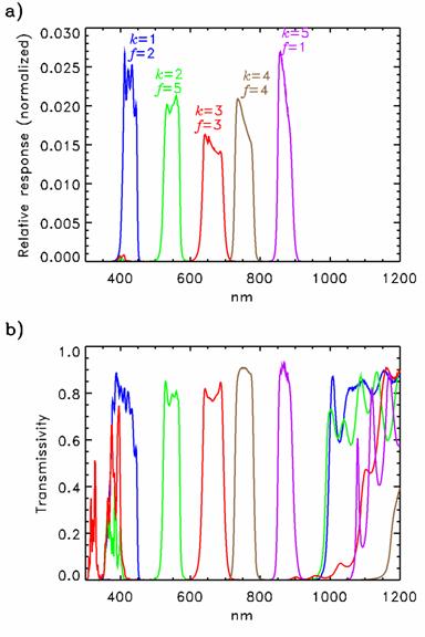
Figure 2. Photograph of the THEMIS-VIS detector and color filter array prior to THEMIS instrument assembly. Band (k) and filter (f) numbers are shown.

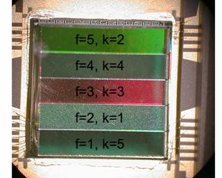
Figure 3. The individual exposures (a) that are used to construct THEMIS-VIS images for each band (b). Both the individual exposures and the assembled images for each band are THEMIS-VIS RDR framelets map projected onto a simple cylindrical coordinate surface, with north at the top and east at right. Each exposure in the time sequence is labeled with its exposure number, a. Each band is labeled with its band number, k. In the time sequence, each framelet is labeled with its framelet number, m, and its band number, k; and in the assembled images, each framelet is labeled with its framelet number, m, and its exposure number, a. For the individual exposures, the area shown for a = 1 to 5 corresponds to the top portion of the assembled images, and the area shown for a = 14 and up corresponds to the bottom portion of the assembled images. The a = 0 exposure is not shown because, as is often the case, a = 0 contains no valid data.

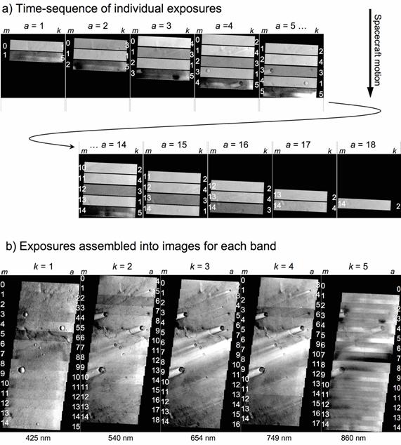
Figure 4. A THEMIS-VIS EDR for the same image as in Figure 3, with the five planes of the EDR layed out from left to right. To display this EDR data, we have performed the 8-bit to 11-bit conversion as described in the text and then applied a linear stretch to the DN values with the limits shown. We indicate filter number f and band number k for each band, and the colored boxes and labels indicate the exposure number a from which particular framelets were extracted.

Figure 5. The hypothesized path followed by the stray light that reaches both the photosites and registers. The dashed line indicates one of many similar paths in which light reaching the edges of the detector is scattered under the edges of the filters. The diagram is not to scale.

Figure 6. Pre-flight test-mode image showing the photosite signal from the integrating sphere calibration source (using nine 8 W lamps), with each filter labeled with its filter (f) and band (k) number. The large boxes outline the regions of the detector from which the 1024 x 192 framelets for each filter are extracted. The smaller boxes show the boundaries of the “calibration region of interest” (C-ROI) for each filter. The inter-filter differences in brightness are due to the spectrum of the light source and the transmissivities of the filters. However, all of the obvious intra-filter non-uniformity in this image is attributable to photosite stray light. This photosite stray light forms the broad stripes on the left and right side of all of the filters as seen in this image. It also forms the bright stripe that covers the bottom half of the f = 1 filter.

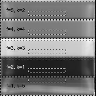
Figure 7. Photosite signal as a function of column in the pre-flight test mode image in Figure 6. The signal for each band is color coded, with blue, green, red, brown, and purple corresponding to k = 1, 2, 3, 4, and 5 (425, 540, 654, 749, and 860 nm), respectively. The column signal is averaged over the rows included in each band’s C-ROI, and is shown as the difference between the column signal and the given band’s C-ROI mean. The vertical lines indicate the boundaries of the C-ROIs (which are identical in the column dimension for all 5 bands).

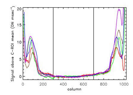
Figure 8. Register signal (solid lines) and photosite signal (dashed lines) as a function of row number, for a 3 msec exposure using pre-flight test-mode and nine 8 W lamps. The signal is averaged over all columns included in the C-ROIs. The shaded regions indicate the rows from which the framelets are extracted, and the darker shaded regions indicate the rows included in each C-ROI. Each shaded region is labeled with its filter (f) and band (k) numbers.

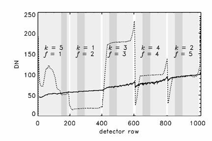
Figure 9. Pre-flight test-mode image showing the register signal from the integrating sphere calibration source (using nine 8 W lamps), with each filter labeled with its filter (f) and band (k) number. The large boxes outline the regions of the detector from which the 1024 x 192 framelets for each filter are extracted. The smaller boxes show the boundaries of the C-ROI for each filter.

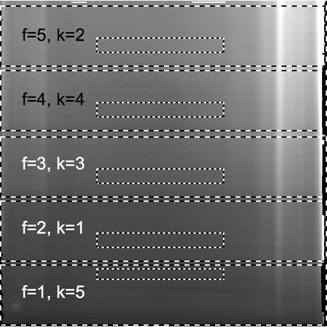
Figure 10. Relative response function of the THEMIS-VIS system excluding the filter transmissivities, i.e., the broadband response function. The response function is normalized so that the area under the curve equals one.

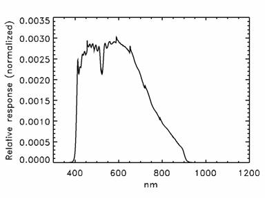
Figure 11. Spectral radiance of the integrating sphere calibration source for (bottom to top) six 8 W lamps, seven 8 W lamps, eight 8 W lamps, nine 8 W lamps, one 45 W lamp, and two 45 W lamps. Solid lines are used for the 45 W lamps, and dashed lines for the 8 W lamps.

Figure 12. Two-dimensional probability density functions for the response coefficient fits at four thermal-vac temperatures. The PDFs are color coded, with blue, green, red, brown, and purple corresponding to k = 1, 2, 3, 4, and 5 (425, 540, 654, 749, and 860 nm), respectively. The contour lines represent c² probabilities of 0.05, 0.30, 0.60, and 0.90.

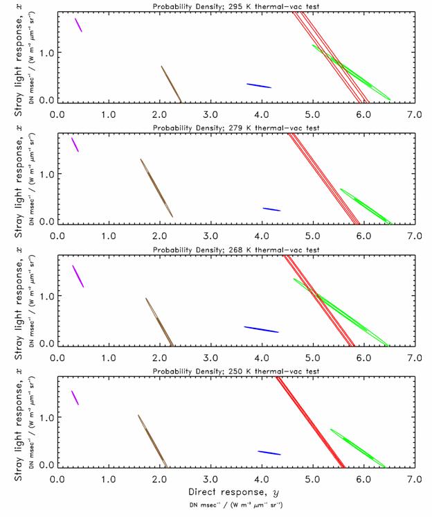
Figure 13. One-dimensional probability density functions for y_k, the direct response coefficients. The PDFs are color coded, with blue, green, red, brown, and purple corresponding to k = 1, 2, 3, 4, and 5 (425, 540, 654, 749, and 860 nm), respectively. Dashed lines show the adopted y values, which correspond to the mean of each PDF. The adopted confidence intervals for y encompass 95% of the total probability and are centered on the PDF mean. The filled regions of each PDF represent regions outside of the adopted confidence intervals.

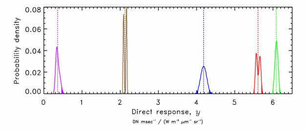
Figure 14. One-dimensional probability density functions for x, the stray light response coefficients. The PDFs are color coded, with blue corresponding to k = 1, and purple corresponding to k = 5. Dashed lines show the adopted x values, which correspond to the mean of each PDF. The adopted confidence intervals for x encompass 95% of the total probability and are centered on the PDF mean. The filled regions of each PDF represent regions outside of the adopted confidence intervals.

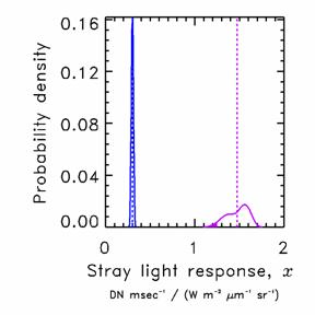
Figure 15. A THEMIS-VIS EDR, as in Figure 4, but of a zero-exposure-time in-flight image.

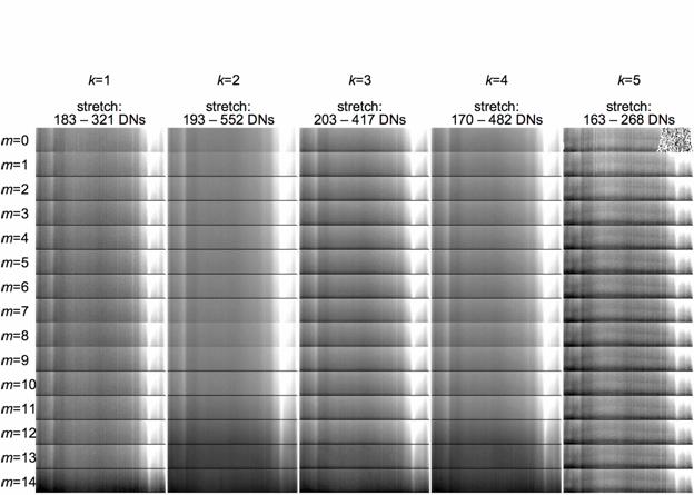
Figure 16. Responsivity, R_ij, as a function of row for filter f = 3 (band k = 3), summing mode 2. The dashed lines are generated by averaging groups of 10 columns. These groups of columns are 210-219, 240-249, 270-279, … 390-399. The bold solid line is the adopted solution for R_j. All lines have been scaled by a common normalization factor, such that R_j, has a mean value of 1 over the rows of the C-ROI.

Figure 17. The C-ROI mean radiance in THEMIS-VIS framelets, plotted against the photometrically corrected radiance measured in concurrent HST images. The data points are color coded, with blue, green, red, brown, and purple corresponding to bands k = 1, 2, 3, 4, and 5 (425, 540, 654, 749, and 860 nm), respectively. A solid line with zero intercept and a slope of one has been drawn in order to highlight the location of points for which the HST and THEMIS-VIS radiances are exactly equal. The left and right-hand plots are identical, except for the range of the axes. None of the k = 1 data points fall within the range of the right-hand plot’s axes.

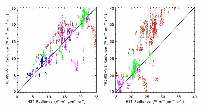
Figure 18. C-ROI register stray light signal as determined by the calibration pipeline for the HST-concurrent data set. The left hand panel shows the relative register signal as a function of effective exposure time for all five bands, using the same color coding as in Fig. 17 (blue, green, red, brown, and purple correspond to the 425, 540, 654, 749, and 860 nm bands, respectively). The right hand panel shows histograms of the same data points after the 1 / effective exposure time scaling factor has been removed. The effective exposure time is the actual exposure time multiplied by the spatial summing mode. The histograms are normalized so that the area under the histogram curve is equal to one. (Note that the histogram for the 860 nm band falls entirely beyond the range selected for the histogram plot).

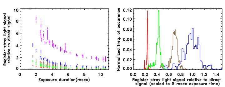
Figure 19. Histogram of the C-ROI photosite stray light signal as determined by the calibration pipeline, presented as a fraction of the direct C-ROI signal determined by the calibration pipeline, for the HST-concurrent data set. Color coding is the same as in Fig. 17 (blue, green, red, brown, and purple correspond to the 425, 540, 654, 749, and 860 nm bands, respectively). The two panels are identical, except for differing x-axis ranges. The histograms are normalized so that the area under the histogram curve is equal to one.

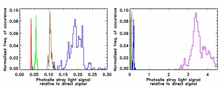
Figure 20. Contour plots of the pixel-dependent component of register stray light, for use in estimating errors in the calibrated C-ROI radiance based on the magnitude of visible artifacts, as discussed in the text. We show this pixel dependent component for a subset of the 31 summing mode 2 register stray light calibration frames. The values plotted are the difference between the register stray light frame and its C-ROI mean, as a fraction of it’s C-ROI mean.

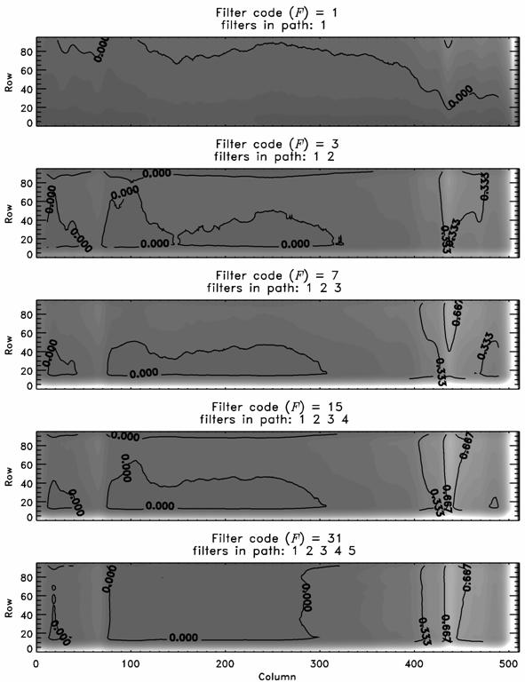
Figure 21. Contour plots of the pixel-dependent component of photosite stray light, for use in estimating errors in the calibrated C-ROI radiance based on the magnitude of visible artifacts, as discussed in the text. We show all 5 summing mode 2 photosite stray light frames. The values plotted are the photosite stray light frame as a fraction of the photosite stray light response coefficient, x.

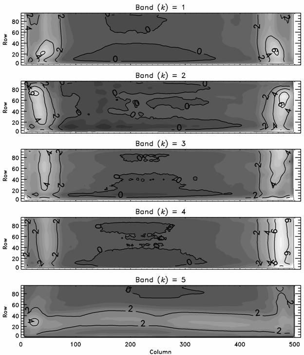
Figure 22. An example RDR with severe register stray light residuals. (Image number V12386007)

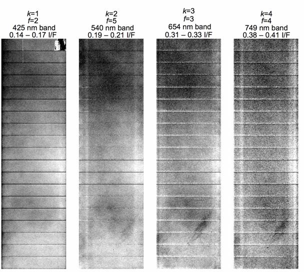
Figure 23. An example RDR with severe photosite stray light and register stray light residuals. (Image number V02699003)

Figure 24. Simple cylindrical, 1 pixel-per-degree projection of HST 763 nm imaging from March 3, 1997 (see Table 3 for details), showing the location of HST pixels used for comparison with THEMIS-VIS spectra in Figs. 26, 28, and 30. The HST data used for these comparisons are not photometrically corrected, which leaves visible seams when the images are mosaiced together.

Figure 25. Sinusoidal projection of THEMIS-VIS image V04289003 with exaggerated colors. North is at the top, and east is at right. The band 1, 2, and 3 images are used for the blue, green, and red channels, respectively, with each channel stretched arbitrarily to maximize contrast. Spectra from regions A and B are shown in Fig. 26. These regions are centered at: A: 29.54° N, 148.48° E, incidence angle 64°; B: 31.69° N, 148.80° E, incidence angle 64°.

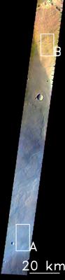
Figure 26. HST WFPC2 and THEMIS-VIS (thick lines) I/F normalized to 1 at ~750nm. The THEMIS-VIS spectra are from V04289003, and their labels correspond to the A and B regions in Fig. 25. The HST spectra, labeled by their latitudes 29 N and 25 N, correspond to the two points labeled with “V04289003” in Fig. 24. The THEMIS-VIS error bars show the standard deviation of I/F in the region from which the spectra were derived.

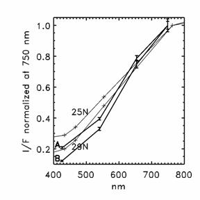
Figure 27. Portion of THEMIS-VIS image V12518004, with sinusoidal projection and exaggerated colors (using bands 1, 2, and 3) as in Fig. 25. Spectra from regions A and B are shown in Fig. 28. These regions are centered at: A: 41.44° N, 44.66° E, incidence angle 68°; B: 41.78° N, 44.70° E, incidence angle 68°.

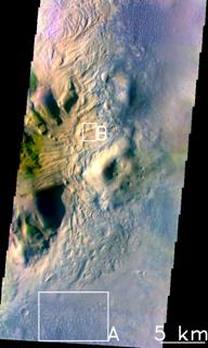
Figure 28. HST WFPC2 and THEMIS-VIS (thick lines) I/F normalized to 1 at ~750nm. The THEMIS-VIS spectra are from V12518004, and their labels correspond to the A and B regions in Fig. 27. The HST spectrum is taken from the point labeled “V12518004” in Fig. 24. The THEMIS-VIS error bars show the standard deviation of I/F in the region from which the spectra were derived.

Figure 29. Portion of THEMIS-VIS image V04984007, with sinusoidal projection and exaggerated colors (using bands 1, 2, and 3) as in Fig. 25. Spectra from regions A and B are shown in Fig. 30. These regions are centered at: A: 60.02° N, 272.73° E, incidence angle 69°; B: 60.07° N, 272.72° E, incidence angle 69°.

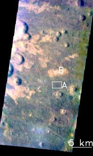
Figure 30. HST WFPC2 and THEMIS-VIS (thick lines) I/F normalized to 1 at ~750nm. The THEMIS-VIS spectra are from V04984007, and their labels correspond to the A and B regions in Fig. 29. The HST spectrum is taken from the point labeled “V04984007” in Fig. 24. The THEMIS-VIS error bars show the standard deviation of I/F in the region from which the spectra were derived.

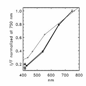
Figure 31. Portion of THEMIS-VIS image V10792003, with sinusoidal projection and exaggerated colors (using bands 1, 2, and 3) as in Fig. 25. Spectra from regions A and B are shown in Fig. 32. These regions are centered at: A: 14.548° S, 175.514° E, incidence angle 75°; B: 14.520° S, 175.571° E, incidence angle 75°. The cross marks the MER-Spirit landing site at 14.5692° S, 175.4729° E (Squyres et al., 2004a).

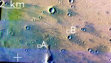
Figure 32. MER-Pancam and THEMIS-VIS (thick lines) I/F normalized to 1 at ~750 nm. The THEMIS-VIS spectra are from V10792003, and their labels correspond to the A and B regions in Fig. 31. The Pancam spectra show a soil and a rock surface near the Spirit landing site, and are taken from Fig. 6C in Bell et al. (2004a). For both data sets, the error bars show the standard deviation of I/F in the region of the image from which that spectrum was derived.

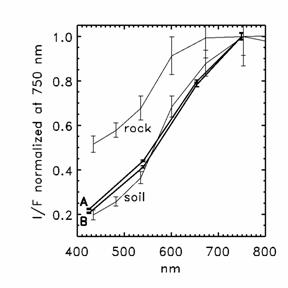
Figure 33. Portion of THEMIS-VIS image V03671001, with sinusoidal projection and exaggerated colors (using bands 1, 2, and 3) as in Fig. 25. Spectra from regions A and B are shown in Fig. 34. These regions are centered at: A: 1.888° S, 354.405° E, incidence angle 71°; B: 2.040° S, 354.370° E, incidence angle 71°. The cross marks the MER-Opportunity landing site at 1.9462° S, 354.4734° E (Squyres et al., 2004b).

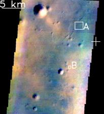
Figure 34. MER-Pancam and THEMIS-VIS (thick lines) I/F normalized to 1 at ~750 nm. The THEMIS-VIS spectra are from V03671001, and their labels correspond to the A and B regions in Fig. 33. The Pancam spectra labeled 1, 4, and 5 correspond to the labels in Bell et al.’s (2004c) Fig 8A. These Pancam spectra show a bright outcrop (1), dark plains (4), and the Eagle crater soil (5). For both data sets, the error bars show the standard deviation of I/F in the region of the image from which that spectrum was derived.